Choose “Save as PDF” in the print dialog, and uncheck “Headers and footers”
so the browser’s URL and date do not stack on the page numbers.
Fluid Mechanics for Atmosphere and Ocean Scientists
Milan Curcic
For Chris Piasecki, who understood the word “ocean”
Front matter
Preface
This book grew out of lecture notes for a graduate-level fluid mechanics course
that I teach at the University of Miami’s Rosenstiel School of Marine,
Atmospheric, and Earth Science.
The course provides advanced undergraduate students or beginning graduate
students with a solid foundation in fluid mechanics concepts that are essential
for understanding ocean physics.
While there are many excellent fluid mechanics textbooks available, most are
written for either for engineering students with a focus on industrial
applications, or for students of meteorology and oceanography that focus on
geophysical flows.
Many of our students at Rosenstiel go on to pursue research topics related to
turbulence, boundary layers, and ocean surface waves, and these topics are well
covered by different textbooks in these respective subdisciplines.
This book bridges that gap by presenting a concise yet comprehensive treatment
of classical, geophysical, turbulent, and wavy fluid mechanics processes
that are relevant to atmospheric and ocean physics research.
The book progresses from fundamental concepts to increasingly complex topics.
We begin with a review of vector calculus before introducing core fluid
mechanics principles such as conservation of mass and momentum.
The effects of Earth’s rotation and density stratification,
which are crucial for atmospheric and ocean dynamics, come next.
We then explore simplified yet powerful models like the shallow water equations
which allow an analytical examination of most common solutions.
Later chapters cover turbulence, boundary layers, and surface gravity waves -
phenomena that are ubiquitous in the ocean and that are becoming increasingly
important in coupled weather-ocean prediction and climate projections.
I aim to balance mathematical rigor with physical intuition throughout the text.
Detailed derivations are provided, but equal emphasis is placed on
understanding the underlying physics.
Examples and figures help illustrate key concepts.
This textbook is a work in progress and continues to evolve.
I welcome feedback from students and colleagues on how to best improve it.
I thank my students Stephen Casey, Katia Childs, Katelyn DeWater,
Susan Harrison, Jack Lee, Ryland Lewis, Kayla Thompson, Joseph Unsworth,
Mia Vallee, and Jessie Yang for their contributions so far.
Special thanks to Prof. Mike Brown who previously taught this course and who
gave me valuable advice on preparing for it.
My hope is that this textbook will serve as a useful resource for students
beginning their journey into atmospheric and/or ocean physics research.
Chapter 1
Introduction
What will you learn in this course
The course aims to provide students with a solid understanding of key fluid
mechanics concepts that are used in ocean physics research.
This course will first refresh you on the vector calculus needed to understand
fluid mechanics, and introduce the Eulerian and Lagrangian views of the flow.
We then proceed to derive the conservation equations for mass and momentum.
We will then consider the effects of rotation and stratification, and look
at some steady solutions of the rotating Navier-Stokes equations.
Then, we will simplify the flow by looking at it as a thin layer of
incompressible rotating fluid that flows over a variable bottom topography
and a free surface.
From there, we will study turbulence and boundary layers, and complete the
course with the linear theory of surface gravity waves.
By the end of the course, you will be proficient in applying fluid mechanical
concepts and mathematical tools to solve many ocean physics research problems.
It will also prepare you for more specialized courses on turbulence, waves,
and atmospheric and oceanic circulation.
Reference textbooks
No single textbook out there covers all the topics that we need for this course.
However, parts of this course are covered in detail by various textbooks.
These lecture notes are based on the following textbooks:
Fluid Mechanics, 7th Ed., by Kundu, Cohen, Dowling, and
Capecelatro (Elsevier), for the classical (Kundu et al., 2024);
Atmospheric and Oceanic Fluid Dynamics (AOFD)
by Geoffrey Vallis (Cambridge University Press),
for the geophysical (Vallis, 2017);
but see also his more concise Essentials of Atmospheric and Oceanic Dynamics (Cambridge University Press),
for a shorter and more selective treatment (Vallis, 2019);
Turbulent Flows by Stephen Pope (Cambridge University Press),
for the turbulent (Pope, 2001);
Water Wave Mechanics for Engineers and Scientists by Dean and
Dalrymple (World Scientific), for the wavy (Dean and Dalrymple, 1991).
While the notes contain the distilled and required information for you to
succeed in this course, please refer to these textbooks for more detailed
explanations and examples.
Over time, the lecture notes will evolve toward a unified, coherent, and
self-contained book.
Chapter 2
Review of vector calculus
In this section we will review the necessary concepts from vector calculus that
we will use in this course.
These include:
scalars, vectors and tensors;
gradient, divergence, and curl;
line, surface, and volume integrals;
and the Gauss and Stokes theorems.
Scalars, vectors, and tensors
In this book we will use three types of quantities to describe fluid
properties: scalars, vectors, and tensors.
Scalars are completely described by their magnitude.
Examples of scalars are temperature, pressure, or density.
A value of 290 K, for example, completely describes the temperature of a fluid
at some point in space and time.
The fundamental scalar fields in fluid mechanics are the pressure, density,
and in some derivations, the velocity potential.
In the atmosphere, density is often represented with the air temperature and
humidity scalars through the ideal gas law.
In the ocean, density if typically represented with the water temperature and
salinity scalars through the equation of state.
The fundamental scalars for us are then, in this approximate order,
pressure, density, temperature, water salinity, and air humidity.
In equations, we will write scalars using italics, e.g.T, p, or ρ.
Vectors have a magnitude and a direction.
Examples of vectors are velocity, acceleration, or force.
In 3-dimensional Cartesian space with coordinates (x,y,z), for example,
vector u(x,y,z) can be described by its components
u=uxuyuz(2.1)
where ux, uy, and uz (each a scalar) are the components of u
in the x, y, and z directions, respectively.
This is the general conventional notation, however, we will often write vectors
inline as u=(u,v,w).
The fundamental vector field of fluid mechanics is the velocity.
Many other vector fields are derived from velocity, such as vorticity,
acceleration, and force.
In equations, we will write vectors using boldface, e.g.u,
a, or F.
The magnitude, or norm, of a vector
u is written as ∣∣u∣∣ and calculated as
∣∣u∣∣=u2+v2+w2(2.2)
Here we’re working in 3-dimensional Cartesian space, but vectors can be defined
in any number of dimensions, and the above definitions generalize exactly how
you’d expect them to.
The most ubiquitous vector field in fluid mechanics is the velocity.
In atmospheres and oceans, we will often refer to the velocity as wind and
current, respectively.
Wind speed is thus the magnitude (norm) of the wind vector, and likewise for
the current speed.
Tensors have magnitude, direction, and orientation.
They are vectors that act on each respective surface orthogonal to the direction
of the tensor.
Arguably the most important tensor in fluid mechanics is the stress tensor.
In 3-dimensional space, for example, a stress tensor can be described as:
τ=τxxτyxτzxτxyτyyτzyτxzτyzτzz(2.3)
In this notation and index ordering, i.e. τij, the first index (i)
refers to the direction of the stress component, and the second index (j)
refers to the direction of the normal to the surface.
In other words, each row of the tensor contains the three components of a
vector, and each column contains the three surface normals that the stress
component is acting on.
For example, τxy is the stress in the x-direction and is acting on the
surface whose normal is in the y-direction (and which lies in the x-z plane).
One special type of tensor is the identity tensorI, which is a tensor that maps a vector onto itself.
In Cartesian coordinates, it is given by:
I=100010001(2.4)
It may be useful to think of scalars as 0th-order tensors, vectors as
1st-order tensors, and tensors as 2nd-order tensors.
Unit vectors
Unit vectors are vectors with magnitude of 1.
A popular notation for unit vectors in Cartesian coordinates is i,
j, and k, which point in the x, y, and z directions,
respectively.
So, a vector u can be written as
u=uxi+uyj+uzk(2.5)
Notice that you can get the unit vector by dividing any vector by its
magnitude, i.e. u/∣∣u∣∣.
Vector operations
Two vectors can be added, subtracted, or multiplied.
Although vector addition and subtraction are straightforward (simply add or
subtract each of their respective scalar components), vector multiplication is
more interesting.
There are many ways to multiply two vectors, but the two most important ones for
us are the dot product and the cross product.
Dot product
The dot product of two 3-dimensional Cartesian vectors
a and b is an element-wise sum of their components
(and thus, a scalar!):
More generally, the dot product of two n-dimensional vectors a and
b is
a⋅b=i=1∑naibi=a1b1+a2b2+…+anbn(2.7)
The dot product is commutative, meaning that
a⋅b=b⋅a.
The magnitude of a dot product of two vectors is equal to the product of their
magnitudes and the cosine of the angle θ between them:
a⋅b=∣∣a∣∣∣∣b∣∣cosθ(2.8)
To visualize this relationship, take one vector and project it onto the other.
This projection is the magnitude of the vector times the cosine of the angle
between them.
Now, one vector and the projection of the other onto the first vector are
pointing in the same direction, so their dot product is the product of their
magnitudes.
It can be useful to think of a dot product as collapsing the two vectors into a
single scalar that contains contributions from each of their components.
The following listing shows how to manually compute the dot product of two
vectors in Python using the built-in arithmetic operators:
import numpy as np# initialize two vectors; specific values are arbitrary.a = np.array([1, 2, 3])b = np.array([4, 5, 6])c = 0 # initialize the result variablefor i in range(a.size): # loop over indices of the vector c += a[i] * b[i] # multiply elements and add to the result
Notice that this an exact implementation of the right-hand side of Eq.
(2.7).
The NumPy library, however, allows element-wise multiplication of vectors,
which is both more computationally efficient and more concise:
c = np.sum(a * b) # multiply element-wise and sum up the components
Notice that this is an exact implementation of the middle part of Eq.
(2.7).
Even though the dot product is simple to implement, as we did above, NumPy
provides a function that is even more concise, and likely the most efficient
way to compute the dot product:
c = np.dot(a, b)
Although it’s important to understand how to implement the fundamental vector
operations by hand, and do it yourself at least once, in practice it’s best to
use established libraries such as NumPy, as they are well tested and optimized
for computational efficiency.
Cross product
The cross product of two vectors a and
b is defined as:
a×b=detiaxbxjaybykazbz(2.9)
where det(M) means the determinant of matrix M.
Using the so-called rule of Sarrus, the cross product can be calculated
as:
The result of a cross product is a vector that is orthogonal to both a
and b.
Its orientation in space is determined by the right-hand rule:
if you point your right thumb in the direction of a and your index
finger in the direction of b, then your middle finger will point in
the direction of a×b.
The magnitude of the cross product is equal to the product of the magnitudes of
the two vectors times the sine of the angle between them:
∣∣a×b∣∣=∣∣a∣∣∣∣b∣∣sinθ(2.12)
So, the magnitude of the cross product is largest when the two vectors are
orthogonal.
Unlike the dot product, the cross product is anticommutative, meaning that
a×b=−b×a.
In fluid mechanics, a cross product will often come up when we are interested in
the rotation of a vector field.
For example, vorticity is the curl of the velocity field.
Matrix multiplication
Occasionally, we will need to multiply a vector by a matrix, or, a matrix by a
matrix.
As a vector is a special case of a matrix in which either the number of rows or
columns is 1, the same rules of matrix multiplication will apply when we
multiply a vector by a matrix or a matrix by a matrix.
These operations are not commutative, meaning that the order of multiplication
matters.
Take two matrices A and B such that
A=a11a21a31a12a22a32a13a23a33(2.13)
and:
B=b11b21b31b12b22b32b13b23b33(2.14)
The result of their multiplication is a matrix C given by:
That is, the entry cij of the product is obtained by multiplying
term-by-term the entries of the i-th row of A and the j-th column
of B, and summing these products.
In other words, cij is the dot product of the i-th row of A
and the j-th column of B.
Although the matrices are not required to be square, the number of columns
of A must be equal to the number of rows of B.
Total and partial derivatives
We will denote total and partial
derivative operators (for example, in time t)
as dtd and ∂t∂.
Scalars, vectors, and tensors alike can be differentiated with respect to any
variable.
A derivative of a vector is simply a vector of derivatives of its components:
Now, we introduce another operator that builds on top of previous
concepts to describe how scalar and vector fields vary in space.
This operator is called del and is denoted by the symbol
∇ (pronounced “nabla”):
∇=∂x∂i+∂y∂j+∂z∂k(2.18)
Written as above, ∇ cannot stand on its own but must be applied as an
operator to a field.
A good way to think about ∇ is as of a differential operator,
which itself is a 3-dimensional vector that can operate on scalars or vectors.
Specifically:
∇p is as vector that is a gradient of a scalar field p;
it quantifies how p changes in space.
∇⋅u is a scalar that is the divergence of a vector
field u; it quantifies how u flows out of a point.
∇×u is a vector that is the curl of a vector field
u; it quantifies how u rotates around a point.
Although, strictly speaking, one is a symbol and the other is an operator,
∇ (“nabla”) and “del” are often used interchangeably when reading equations
out loud.
Gradient
The gradient of a scalar field T is a vector field that points in the
direction of the greatest rate of increase of T.
It is denoted by ∇T and is defined as
∇T=∂x∂Ti+∂y∂Tj+∂z∂Tk(2.19)
Gradient of a scalar field is a vector that points in the direction of the
steepest increase of that field, and its magnitude is the rate of that increase.
Imagine hiking up a hill; the gradient of the terrain is a vector
that is pointing toward the steepest incline, and its magnitude is the steepness
of that incline.
Hover or tap the field below to read T and see ∇T:
the arrow is orthogonal to the isolines and points uphill.
Divergence
The divergence of a vector field u is a scalar field that describes
the rate at which the vector field flows out of a point.
It is denoted by ∇⋅u and is defined as
∇⋅u=∂x∂ux+∂y∂uy+∂z∂uz(2.20)
Divergence of a vector field is a scalar that describes how much the vector
field is expanding or contracting at a point.
Negative divergence is called convergence.
The explorer below colors the plane by ∇⋅u and draws
u as arrows: spreading arrows and warm colors are sources;
converging arrows and cool colors are sinks.
Curl
The curl of a vector field u is a vector field that describes the
rotation of the vector field.
It is denoted by ∇×u and is defined as
Curl of a vector field is another vector that is orthogonal to the original
vector field and quantifies how much the vector field is rotating around a
point.
When curl is zero, the vector field is said to be irrotational.
In two dimensions the curl is out of the plane, (∇×u)z.
The paddle wheel below spins with that local rotation; shear is a reminder
that curl need not look like a vortex.
Laplacian
The Laplacian is a second-order differential operator that
can be applied to both scalar and vector fields.
It measures the rate at which field varies in space and is defined as:
∇2=∂x2∂2+∂y2∂2+∂z2∂2(2.22)
Applied to a scalar field T, it is:
∇2T=∂x2∂2T+∂y2∂2T+∂z2∂2T(2.23)
Applied to a vector u=(u,v,w), it is applied to each component:
The Laplacian of a scalar is thus a scalar and the Laplacian of a vector is a
vector.
In some literature you will see the Laplacian written as Δ, but here we
will use ∇2 to avoid confusion with the Δ that we use to denote
a finite increment.
Useful vector identities
Curl of a gradient of a scalar field is always zero:
∇×(∇T)=0(2.25)
Further, divergence of a curl of a vector field is always zero:
∇⋅(∇×u)=0(2.26)
Finally, curl of a curl of a vector field is:
∇×(∇×u)=∇(∇⋅u)−∇2u(2.27)
Some of these identities will come handy when we derive the conservation of
vorticity laws.
Gauss and Stokes theorems
The most useful in our work will be variants of the
Gauss and Stokes theorems.
The Gauss theorem relates a volume integral of a divergence of a vector field
to a surface integral of that vector field.
The Stokes theorem relates a surface integral of the curl of a vector field to
a line integral of that vector field.
Here, they are stated for reference, and we’ll explore their meaning and
application in more detail as we use them to derive the fundamental equations
for fluid flows.
Gauss theorem
The Gauss theorem states that the volume integral of the
divergence of a vector field u over a volume V is equal to the
surface integral of u over the surface A that encloses V:
∫V∇⋅udV=∮Au⋅dA(2.28)
In other words, the rate of change of the fluid mass within a volume is equal to
the flow normal through the surface that encloses that volume.
This form of Gauss’s theorem is also known as the
divergence theorem.
It will come in handy when we derive the conservation of mass (continuity)
equation.
Stokes theorem
The Stokes theorem states that the surface integral of the curl of a
vector field u over a surface A is equal to the line integral of
u over the boundary of A:
∫A(∇×u)⋅dA=∮∂Au⋅dl(2.29)
In other words, the rotation rate of the fluid over a surface area is equal to
the flow velocity integrated around the boundary of that surface.
Summary
In this chapter, we reviewed:
Scalars, vectors, and tensors;
Vector algebra: dot product (a⋅b) and cross
product (a×b);
Derivatives: total (dtd) and partial (∂t∂);
Gradient, divergence (∇⋅u), and curl (∇×u);
Gauss theorem that relates volume and surface integrals:
∫V∇⋅udV=∮Au⋅dA;
Stokes theorem that relates surface and line integrals:
∫A(∇×u)⋅dA=∮∂Au⋅dl.
These concepts will serve as the basic building blocks for everything that
follows in the remainder of this course.
Exercises
Pick your favorite programming language (or ask for a recommendation for one).
Write a program that defines a scalar, a vector, and a tensor, and assign
numerical values to them.
Print the values to the screen.
Is there a difference in how you define them in your program?
What is the dot product of two orthogonal vectors?
How about the dot product of a vector with itself?
Please write out the solution step by step.
Write a program that calculates the cross product of two vectors.
Please implement your solution using the basic arithmetic operations such as
addition and multiplication.
Then, see if your programming language or one of its software libraries
provides a function to do this.
Can you verify your implementation by comparing its output to that of the
library function?
How would you calculate a derivative of a quantity
(scalar, for example) in a computer program, e.g. ∂x∂a?
Consider that you can approximate a derivative as a difference between two
values of the quantity at two points in space.
In other words, assume ∂a≈Δa=a(x2)−a(x1),
and similar for x.
Write a computer program that calculates the gradient of a scalar field,
and the divergence and curl of a vector field.
Draw example vector fields that are: (a) non-divergent and irrotational,
(b) divergent and irrotational, (c) non-divergent and rotational, and (d)
divergent and rotational.
import numpy as np
import matplotlib.pyplot as plt
#
# Try the programming exercises above in this Python session.
# NumPy and Matplotlib are already available.
#
# 1. Define a scalar, a vector, and a tensor, then print them.
# 3. Compute a cross product by hand, then with a library function.
# 4. Approximate a derivative with finite differences.
# 5. Compute the gradient of a scalar field, and the divergence and curl
#    of a vector field.
# 6. Plot example vector fields with plt.quiver.
Chapter 3
Fluid kinematics
Fluid kinematics describe the fluid motion without considering the forces that
cause that motion.
We will explore two main views of the flow: the Lagrangian
view, which follows individual fluid particles, and the Eulerian
view, which observes the flow at fixed points in space.
Although the Eulerian (fixed-point) view is more commonly used in the theory and simulation
of fluid flows, the Lagrangian (particle-following) view will be essential when
deriving some of the fundamental equations, as well as for understanding where
certain features of the flow come from.
Both approaches are often used together in numerical simulations.
Flows are typically simulated in the Eulerian framework on a fixed
grid, and for many applications the flow is analyzed a posteriori
and/or visualized in the Lagrangian framework.
For example, picture a high-speed flow simulation around an aircraft
that is modeled on a fixed grid, and particle-following trajectories drawn to
visualize the turbulent wake behind the vessel.
Another example is the Lagrangian evolution of an oil spill in the ocean or
a volcanic plume in the atmosphere, derived from Eulerian simulation output.
We will also introduce some useful concepts to describe the flow, namely
the velocity potential and the stream function.
These two scalar quantities are complementary to the vector field of velocity
and together provide a complete description of the flow.
Lagrangian and Eulerian derivatives of a fluid property
We will start by first drawing a distinction between the Lagrangian and Eulerian
derivatives.
Consider a 3-dimensional quantity φ that varies in space and time such
that φ=φ(x,y,z,t).
This can be a scalar, a vector, or a tensor, however, to keep things simple,
suppose φ is a scalar field.
Let’s find its rate of change.
Since it depends on x, y, z, and t, the rate of change of φ along
each of these dimensions must be taken into account.
So, the total change of φ (let’s call it δφ, where δ
is a small but finite increment) over spatial and temporal increments δx,
δy, δz, and δt, is the sum of changes along each of
these dimensions:
δφ=∂x∂φδx+∂y∂φδy+∂z∂φδz+∂t∂φδt(3.1)
Divide by δt to obtain:
δtδφ=∂x∂φδtδx+∂y∂φδtδy+∂z∂φδtδz+∂t∂φ(3.2)
Recall the definition of ∇ (Eq. 2.18) and let the finite
increment δt approach dt (and likewise for δx, δy, and
δz), to obtain:
dtdφ=∂x∂φdtdx+∂y∂φdtdy+∂z∂φdtdz+∂t∂φ(3.3)
The above is equivalent to applying the chain rule to φ with respect
to time and assuming that the spatial dimension variables are functions of time
(φ=φ(x(t),y(t),z(t),t)).
Recognize that by stating the dependence of position on time, we are implicitly
stating that we are following a fluid particle.
Then, recognize that the velocity in each direction is the rate of change of
the position in that direction:
dtdφ=∂t∂φ+u∂x∂φ+v∂y∂φ+w∂z∂φ(3.4)
which states that the total change of φ is due to the local (at fixed
point in space) change over time, and due to spatial variations of φ as
the fluid particle moves through them.
Finally, recall the definition of ∇ (Eq. 2.18) to obtain:
dtdφ=∂t∂φ+u⋅∇φ(3.5)
The term dtdφ is called the total derivative
of φ. It is also called a Lagrangian derivative,
or material derivative, since it follows
the motion of a fluid particle.
The term ∂t∂φ is called the
Eulerian derivative,
or partial derivative
of φ with respect to time.
The term u⋅∇φ describes how φ changes due
to its spatial variation and the flow of the fluid.
Although the term u⋅∇φ is the dot product of
u and ∇φ, the Lagrangian derivative in Eq.
3.5 can be expressed as an operator:
dtd=∂t∂+(u⋅∇)(3.6)
The parentheses on the right-hand side indicate that that term acts as an
operator on a field.
Like we stated for the operator ∇ in the previous chapter, the total
derivative operator dtd cannot stand on its own, but is instead
applied to a field.
Lagrangian derivative of a volume
Consider a fluid parcel with a constant mass but whose volume may change over
time and is ∫VdV=V.
The total rate of change of that volume as it moves with the fluid is equal to
the surface integral of the velocity field u through the surface
S that is bounding the volume V:
dtd∫VdV=∫Su⋅dS(3.7)
Recall now the divergence theorem (Eq. 2.28) to obtain:
dtd∫VdV=∫V∇⋅udV(3.8)
Now, for a volume parcel so small that ∫VdV=ΔV→0, the
velocity divergence can be considered to be constant over the volume, and the
integral can be replaced by the volume itself:
dtdΔV=ΔV∇⋅u(3.9)
We can derive a similar expression for the rate of change of a fluid property
per unit volume q, such that qΔV is the amount of that quantity in
a fluid parcel with the volume ΔV.
dtd(qΔV)=ΔVdtdq+qdtdΔV(3.10)
Recall the material derivative of ΔV from Eq. 3.9
to obtain:
dtd(qΔV)=ΔVdtdq+qΔV∇⋅u(3.11)
dtd(qΔV)=ΔV(dtdq+q∇⋅u)(3.12)
This was for a fluid property that is defined per unit volume.
Let’s now do the same for some property φ that is defined per unit mass,
such that φρΔV is the amount of that quantity in the fluid
parcel with the volume ΔV and density ρ (and mass ρΔV).
dtd(φρΔV)=ρΔVdtdφ+φdtd(ρΔV)(3.13)
However recall that our fluid parcel has constant mass, so dtd(ρΔV)=0.
Our total derivative becomes:
dtd(φρΔV)=ρΔVdtdφ(3.14)
The Lagrangian derivative of a volume will come in handy when we derive the
continuity equation in the next chapter.
Velocity potential
Velocity potential is defined as a scalar field ϕ such that the velocity
field u is the gradient of ϕ:
u=∇ϕ=∂x∂ϕ∂y∂ϕ∂z∂ϕ(3.15)
The concept of the velocity potential is useful in fluid mechanics because it is
often easier to work with a scalar field than a vector field.
We will revisit it later in Chapter Surface gravity waves when we
derive the equations of surface gravity waves.
Summary
In this chapter, we covered:
Lagrangian (material) and Eulerian (field) derivatives;
the former follows a fluid parcel of constant mass as it moves through
the flow field, while the latter is the rate of change at a fixed point
(or volume) in space;
The Lagrangian derivative of volume, as well as of a fluid property per
unit volume and per unit mass.
We’ll use these concepts in the next chapter where we derive the equations of
continuity and motion.
Chapter 4
Conservation of mass and momentum
In this chapter we will derive the fundamental equations for fluid flows:
continuity, momentum, and energy.
We start with the conservation of mass, which is the easiest to derive, but also
arguably the most fundamental.
Conservation of mass
Recall from the previous chapter that we can take at least two perspectives
on the fluid flow: the Lagrangian perspective, which follows a fluid parcel as it
moves through space, and the Eulerian perspective, which observes the flow at
fixed points in space.
We can thus derive the conservation of mass, or commonly known as the
continuity, from both perspectives.
Let’s start with the Eulerian perspective, as it may seem more intuitive to
derive from first principles.
Eulerian derivation
Consider a fixed rectangular volume ΔV=ΔxΔyΔz in
three-dimensional space.
The mass of the fluid in this volume is ρΔV, where ρ is the
density of the fluid.
The fluid enters the volume through the surfaces of the box, and the rate at
which the mass enters the volume through a surface is given by the product of
the density, the velocity component normal to the surface, and the area of the
surface.
Let’s call this velocity u with components u, v, and w in the
x, y, and z directions, respectively.
For simplicity, let’s first consider only the x-component of the velocity.
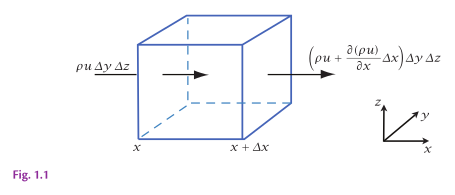
This scenario is illustrated in Fig. 4.1.
The fluid mass flow rate into the volume through the left face is ρuΔyΔz,
and the mass flow rate out of the volume through the right face is
ρ(u+∂x∂uΔx)ΔyΔz.
The net mass increase in the control volume must be governed by the net mass
inflow excess relative to the net mass outflow:
Figure 4.1.
Mass conservation in an rectangular Eulerian control volume. The mass convergence, ∂(ρu)/∂x (plus contributions in the y and z directions), must be balanced by a density decrease. This is Fig. 1.1 in AOFD (Vallis, 2017).
∫V∂t∂ρdV=ρuΔyΔz−(ρu+∂x∂(ρu)Δx)ΔyΔz(4.1)
∫V∂t∂ρdV=−∂x∂(ρu)ΔxΔyΔz(4.2)
Now, if we allow the flow field to have components in the y and z directions
as well, the equation becomes:
∫V∂t∂ρdV=−[∂x∂(ρu)+∂y∂(ρv)+∂z∂(ρw)]ΔV(4.3)
Let ΔV→0 to such that any field within ΔV is uniform to obtain:
∂t∂ρ+∇⋅(ρu)=0(4.4)
This is the continuity equation in the Eulerian reference frame.
Drag the mass-flux arrows on each face of the control volume below.
The local density tendency is minus the sum of the three divergence
contributions.
We’re not constrained to a rectangular, fixed volume, however.
We can derive this equation for an arbitrary control volume using the divergence
theorem.
The total rate of change of that volume as it moves with the fluid is equal to
the surface integral of the velocity field u through the surface
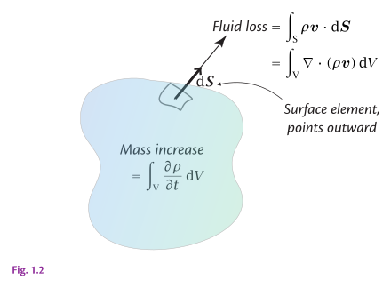
S that is bounding the volume V (Fig. 4.2).
Mathematically, we can express this as:
Figure 4.2.
Mass conservation in an arbitrary Eulerian control volume V bounded by a surface S. The mass increase, ∫V(∂ρ/∂t)dV is equal to the mass flowing into the volume, −∫S(ρv)⋅dS=−∫V∇⋅(ρv)dV. This is Fig. 1.2 in AOFD (Vallis, 2017).
∫V∂t∂ρdV=−∫Sρu⋅dS(4.5)
Now, recall the divergence theorem (Eq. 2.28) to obtain:
∫V∂t∂ρdV=−∫V∇⋅(ρu)dV(4.6)
Let ΔV→0 to integrate and drop ΔV on both sides to obtain
Eq. 4.4, which is the Eulerian form of the continuity
equation.
Lagrangian derivation
In the Lagrangian frame, we follow a fluid parcel as it moves through space.
Its mass ρΔV is constant by definition, but its density or volume
may change.
Since the mass of the parcel is constant, its Lagrangian derivative is zero:
dtd(ρΔV)=0(4.7)
Since the mass doesn’t change, any change in the density of the parcel must be
balanced by a change in its volume:
ΔVdtdρ+ρdtdΔV=0(4.8)
Recall that we’ve already derived the Lagrangian derivative of a volume of the
fluid parcel (Eq. 3.9), which is the second
term here.
The equation becomes:
ΔVdtdρ+ΔVρ∇⋅u=0(4.9)
Finally, drop ΔV on both sides to obtain the Lagrangian form of the
continuity equation:
dtdρ+ρ∇⋅u=0(4.10)
Equations 4.4 and 4.10 are
two fundamental expressions of the conservation of mass for a fluid.
In one form or another, this equation is a critical component of all weather,
ocean, and climate prediction models.
Continuity of an incompressible fluid
Liquids are nearly incompressible, and for them dtdρ=0 is a good
approximation.
For an incompressible fluid, the continuity equation simplifies to:
∇⋅u=0(4.11)
Although as simple as it gets, Eq. 4.11 is
extremely important in fluid dynamics.
Conservation of momentum
Like the conservation of mass, the conservation of momentum is a fundamental
concept in fluid mechanics.
It allows us to predict how the fluid should accelerate due to its state
(i.e. velocity and density) and due to the forces acting on it.
Together, the continuity and momentum conservation
equations form the core of most fluid prediction models, such as weather, ocean,
and climate prediction models.
We will derive the momentum equation in the remainder of this section.
We’ll start from the most basic form first and then incrementally introduce
some common forces, such as the pressure gradient force, gravity, and viscosity.
The first step
To derive the momentum conservation equation, we will start from the second
Newton’s law, which states that the time rate of change of the momentum of a
fluid particle is equal to the net force acting on it.
For a fluid parcel of volume ΔV=∫VdV whose momentum per unit mass
is ρu, the momentum conservation equation is:
dtd∫VρudV=∫VFdV(4.12)
where F is the net force per unit volume acting on the fluid parcel.
Let again the volume parcel be very small such that its density and net force
acting on it are uniform. We have:
ρdtduΔV=FΔV(4.13)
ρdtdu=F(4.14)
Recall the Lagrangian derivative operator from Eq. 3.5
to obtain:
∂t∂u+u⋅∇u=ρF(4.15)
This equation states that the acceleration of a fluid parcel at any fixed point
in space is equal to the net force per unit mass acting on it, divided by the
fluid density.
The second term on the left-hand side is the advection term.
It represents the local acceleration of the fluid parcel due to the properties
of the fluid flow itself.
Consider for example a 1-dimensional flow such that the advection term reduces
to u∂x∂u.
Notice that the advection term is zero only in two special cases:
when the velocity is zero or when the velocity is spatially uniform.
In all other cases the advection term is non-zero and contributes to the local
acceleration.
Because the advection term is velocity multiplied by its gradient, it is
nonlinear.
This single property of this term makes accurate analysis and prediction of
fluid flows difficult.
For example, the nonlinear advection term is responsible for the existence of
chaos in fluid flows, where small differences in initial
conditions lead to vastly different outcomes (in popular culture known as the
butterfly effect).
One consequence of this in our daily lives is that weather predictability
is limited to a finite lead time horizon, for example one to two weeks depending
on the weather patterns of interest.
If, however, we could assume that either the velocity or its gradient are so
small that they could be neglected, the equation simplifies significantly
and often allows for analytical solutions.
u⋅∇u is the most important term for
turbulence, weather prediction and predictability, and a major obstacle toward
analytical solutions of Eq. 4.15 and its variants.
Remember this now.
Back to our equation.
For a 3-dimensional Cartesian flow where the velocity field is u=(u,v,w)
and net forces are F=(Fx,Fy,Fz), Eq. 4.15
becomes a system of three equations, one for each component of the velocity field.
Recall from the Lagrangian derivative operator that u⋅∇u
is an operator acting on u (as opposed to divergence of a gradient).
The u⋅∇ operator then expands to
u∂x∂+v∂y∂+w∂z∂.
Our vector equations becomes a system of three scalar equations:
∂t∂u+u∂x∂u+v∂y∂u+w∂z∂u=ρFx(4.16)
∂t∂v+u∂x∂v+v∂y∂v+w∂z∂v=ρFy(4.17)
∂t∂w+u∂x∂w+v∂y∂w+w∂z∂w=ρFz(4.18)
Each of the prognostic equations for the velocity components thus has exactly
three advective components that correspond to the gradients of the velocity
in each respective direction.
Incorporating the forces
Now we should consider what forces may be acting on the fluid.
We distinguish between two types of forces: surface forces and body forces.
Surface forces act on the surface of the fluid parcel due to the motion of the
fluid molecules, in all directions at that surface.
For example, organized motion of molecules into the surface may cause pressure
on that surface, and the sheared motion of molecules (e.g. if flow is
antiparallel to the surface) may cause shear stress on the surface, leading to
the deformation of the fluid parcel.
In contrast, body forces act remotely (meaning, from a distance) on the entire
volume of the fluid parcel because that parcel is immersed in one or more force fields.
Gravity is one such body force, and it’s the only one we’ll consider here.
Although in Eq. 4.15 we wrote the net force as F,
it’s useful to write it as the sum of body forces Fb and surface
forces Fs:
∂t∂u+u⋅∇u=ρ1(Fs+Fb)(4.19)
Let’s derive the surface forces first.
We want to find out the local change of momentum only due to the surface forces.
Analogous to how the flow through the volume determined the rate of change of
density inside that volume, as we saw in the continuity equation
(Eq. 4.4), the change in momentum inside the volume
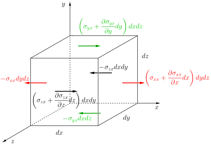
is determined by the surface forces acting on the volume (Fig. 4.3).
where σ is the second-order stress tensor acting on the
surface S of the fluid parcel.
As before, recall the divergence theorem (Eq. 2.28) to obtain:
∫VFsdV=∫V∇⋅σdV(4.21)
Fs=∇⋅σ(4.22)
The surface force thus equals the divergence of the stress tensor.
Insert this into Eq. 4.15 to get our new form of
the momentum equation:
∂t∂u+u⋅∇u=ρ1∇⋅σ+ρFb(4.23)
This form of the momentum equation is often called the
Cauchy momentum equation.
Let’s now look at what this stress tensor divergence term
∇⋅σ is.
Pressure gradient
There is a fundamental difference in the meaning of the diagonal and off-diagonal
components of the stress tensor.
The diagonal components of the stress tensor, σxx, σyy, and
σzz, represent the normal stress components, i.e. the force per unit
area acting on a surface element that is oriented in the x, y, and z
directions, respectively.
The off-diagonal components of the stress tensor represent the shear stress
components, each acting on all three surfaces.
For example, σxy represents the x-component of the stress tensor
acting on the surface that is perpendicular to the y-axis.
Let’s write out the stress tensor in Cartesian coordinates:
σ=σxxσyxσzxσxyσyyσzyσxzσyzσzz(4.24)
This tensor can be decomposed into an isotropic pressure contribution and a
viscous contribution:
σ=−pI+τ(4.25)
where p is the pressure, I is the identity tensor,
and τ is the viscous stress tensor, which can contain both
normal and shear stresses.
For the incompressible Newtonian flow considered below, τ is
also deviatoric, meaning that its trace is zero.
Written out explicitly in Cartesian coordinates and using Eq.
4.25, the stress tensor is:
Let’s insert this into Eq. 4.15 to get our new form of
the momentum equation:
∂t∂u+u⋅∇u=−ρ1∇p+ρ1∇⋅τ+ρFb(4.28)
Pressure is one of the fluid properties that determine its state.
Collective, organized, motion of molecules at a macroscopic scale induces
pressure on a surface and an associated force acting normal to that surface.
Recall that the surface vector is normal to the surface and pointing outward,
and the force acting on the fluid surface is oriented inward, thus the minus sign.
In an ideal, inviscid fluid, that is, a fluid that exhibits no viscous
forces, the stress tensor σ is only composed of the diagonal
terms (pressure). The viscous stress is zero, but the total stress divergence
is −∇p, which need not vanish.
Dropping ∇⋅τ and the body forces Fb for
now, the Cauchy momentum equation simplifies to:
∂t∂u+u⋅∇u=−ρ1∇p(4.29)
This form of the momentum equation is often called the Euler equation.
Viscous forces
Now, let’s look at the viscous stress tensor divergence ∇⋅τ.
Written out explicitly as a matrix of all its components, τ is:
τ=τxxτyxτzxτxyτyyτzyτxzτyzτzz(4.30)
The diagonal components of the viscous stress tensor are the viscous normal stresses,
while the off-diagonal components are the shear stresses.
Viscous normal stresses can be non-zero even in incompressible flow: a fluid
parcel can stretch in one direction while contracting in another without
changing its volume.
In an inviscid fluid, all components of τ vanish.
For an ordinary fluid without couple stresses, angular momentum conservation
requires the stress tensor to be symmetric, so τxy=τyx,
τxz=τzx, and τyz=τzy.
For example, τxy is the force in the x direction per unit area on a
face normal to the y direction. The stress divergence is the vector:
Now, write out 4.28 as a system of three scalar
equations, one for each component of the velocity field, and insert the shear
stress divergence terms to get:
Each of the prognostic equations for the velocity components thus has exactly
one pressure gradient, one viscous normal stress gradient, and two shear stress
gradient terms, all arising from the surface forces.
To express the viscous stress in terms of velocity, we need a
constitutive relation: a model of how the material responds to deformation.
Conservation laws alone do not determine this relation.
Adding a uniform velocity to the whole fluid does not change its deformation
or viscous stress, so the relevant quantity is the relative motion of nearby
fluid particles.
For particles separated by a small vector δx, their velocity
difference is, to first order,
δu≈(∇u)δx.
With velocity components u, v, and w in the x, y, and z directions,
the velocity gradient is the tensor:
The velocity gradient contains both deformation and rigid rotation.
Its symmetric part is the rate-of-strain tensor:
D=21[∇u+(∇u)T](4.36)
Here the superscript T denotes the transpose, which swaps rows and columns.
For example, Dxx=∂u/∂x and
Dxy=Dyx=21(∂u/∂y+∂v/∂x).
The antisymmetric part, 21[∇u−(∇u)T],
describes local rigid rotation, which does not deform the parcel.
For example, rigid rotation u=(−Ωy,Ωx,0), with constant
angular velocity Ω, has a non-zero velocity gradient but D=0.
It therefore produces no Newtonian viscous stress.
For a Newtonian fluid, the constitutive assumption is that viscous
stress depends linearly on the instantaneous local rate of strain.
For an isotropic fluid, whose material properties have no preferred direction,
the general linear relation is
τ=2μD+λ(∇⋅u)I,
where μ and λ are viscosity coefficients and p is the thermodynamic
pressure. In compressible flow, this viscous stress need not be traceless.
From here on, we assume incompressible flow, so ∇⋅u=0 and
the relation reduces to:
τ=2μD=μ[∇u+(∇u)T](4.37)
The coefficient μ is the dynamic viscosity. It depends on the material and
its thermodynamic state, including temperature, but for a Newtonian fluid it
does not depend on the rate of strain.
Experiments establish when this linear model is appropriate and measure μ.
For simple shear, u=(u(y),0,0), this tensor relation gives the familiar
scalar law τxy=τyx=μdu/dy.
It also gives viscous normal stresses such as τxx=2μ∂u/∂x.
For example, u=(ax,−ay,0), with constant a, is incompressible but has
τxx=2μa and τyy=−2μa.
Inserting the incompressible constitutive relation into
Eq. 4.28, we get:
∂t∂u+u⋅∇u=−ρ1∇p+ρ1∇⋅{μ[∇u+(∇u)T]}+ρFb(4.38)
If we also assume that the dynamic viscosity is spatially constant, the viscous
stress divergence simplifies as follows:
∇⋅τ=μ∇2u+μ∇(∇⋅u)=μ∇2u(4.39)
The last equality uses incompressibility. The viscous force is retained;
only the term involving ∇⋅u vanishes.
This gives the incompressible Navier-Stokes equation:
∂t∂u+u⋅∇u=−ρ1∇p+ν∇2u+ρFb(4.40)
where ν=ρμ is the kinematic viscosity.
The operator ∇2=(∂x2∂2+∂y2∂2+∂z2∂2)
is the Laplacian.
It is a second-order differential operator that appears in many partial
differential equations, including the heat equation, the wave equation, and
the Laplace equation.
More on these later.
Let’s now look at the body forces to conclude our derivation.
Gravity
As we mentioned earlier, gravity is the only body force we’ll consider here.
The force of gravity per unit mass is given by g=(0,0,−g),
where g is the gravitational acceleration.
Here we assume that the gravitational acceleration is constant and points downward.
Insert this into Eq. 4.40, and assuming
incompressibility, we get:
∂t∂u+(u⋅∇)u=−ρ1∇p+g+ν∇2u(4.41)
Written out explicitly for each of the three spatial dimensions (x, y, and z),
we get:
This completes the full system of momentum conservation equations in the
Cartesian coordinate system.
Hydrostatic balance
Take Eq. 4.44 and assume that the vertical
acceleration dtdw is small compared to g, and that the spatial
variations of w are small.
We can then drop the dtdw and ν∇2w terms to get the
hydrostatic approximation:
∂z∂p=−ρg(4.45)
which states that the vertical pressure gradient is governed by the density
of the fluid and the gravitational acceleration.
It’s often a good approximation for large-scale atmospheric and oceanic flows,
where the vertical variations of the horizontal velocity components are much
smaller than the horizontal variations of the vertical velocity component.
Notice however that the hydrostatic approximation does not imply that there
is no vertical motion or that it does not vary over time.
Instead, according to the continuity equation (Eq. 4.10),
it means that the vertical motion is completely governed by the change in
density and the divergence of the horizontal velocity field.
Further, if the flow is incompressible (∇⋅u=0),
we get:
∂z∂w=−∂x∂u−∂y∂v(4.46)
which relates the vertical acceleration to the horizontal divergence.
Integrating this equation vertically allows us to calculate the vertical velocity
anywhere in the fluid column provided bottom and top boundary conditions:
w(z)=w(z+Δz)−∫zz+Δz(∂x∂u+∂y∂v)dz′(4.47)
This relationship will prove to be extremely useful in ocean applications where
only the horizontal velocity field is resolved.
For example, a group of ocean surface drifters converging towards a region is
indicative of downwelling (downward motion in the ocean) in that region.
Another example is that of ocean circulation models, which are typically
designed as hydrostatic.
In the case of such models, the horizontal components of the velocity are
prognostic variables, and the vertical velocity is diagnosed using
Eq. 4.46.
Equation of state
Now that we have derived the mass and momentum conservation equations, let’s
write them out together in vector form:
∂t∂u+(u⋅∇)u=−ρ1∇p+g+ν∇2u(4.48)
∂t∂ρ+∇⋅(ρu)=0(4.49)
Momentum and mass conservation equations are prognostic equations for the
vector velocity field u and the scalar density field ρ,
respectively.
Notice the one remaining unknown: the scalar pressure field p.
As of now, we have a system of two independent equations for the three unknowns:
u, p, and ρ.
We need one more equation to close the system—the
equation of state—to relate the pressure to
the other properties of the fluid, such as temperature, density, and
composition.
The prognostic equations that we have derived so far describe equally well
the evolution of both the atmosphere and the ocean, despite their significant
differences.
The equation of state is where our systems of governing equations for the ocean
and the atmosphere begin to diverge.
Namely, the atmosphere is a mixture of dry air and water vapor, and the
ocean is composed of liquid water with varying amounts of dissolved salts.
These differences will reflect in the choice of the equation of state to use
in each of these systems.
In the atmosphere
In the atmospheres, ideal gas law
is often used as the equation of state:
p=ρRT(4.50)
where R is the specific gas constant for the gas in question, and T is the
temperature.
For the moist air, we need to account for both the properties of dry air
(Rd≈287Jkg−1K−1) and those of water vapor
(Rv≈461Jkg−1K−1).
The equation of state for moist air relies on the so-called
virtual temperature to account for the
moisture in the air:
p=ρRdTv(4.51)
where:
Tv=T[1+q(RdRv−1)](4.52)
where q is the specific humidity of the air.
So, the equation of state for moist air is:
p=ρRdT[1+q(RdRv−1)](4.53)
Recall that we intended to close our system of equations by finding the
equation for pressure.
Although we did solve for pressure, it seems that we introduced two new
unknown variables: the temperature T and the specific humidity q.
Each of these variables are governed by their own conservation equations,
akin to that for density, but with the addition of source and sink terms
that control their production and loss:
∂t∂T+(u⋅∇)T=S˙T(4.54)
∂t∂q+(u⋅∇)q=S˙q(4.55)
where S˙T and S˙q are the sources and sinks of temperature and
specific humidity, respectively.
They are governed by a plethora of thermodynamic processes such as radiation,
evaporation, condensation, etc.
Although we won’t delve further into the details behind the sources and sinks
of temperature and specific humidity in the atmosphere, we can denote these
equations as completing the full system of prognostic equations for the
atmosphere: Eqs. 4.48,
4.49,
4.53,
4.54, and
4.55.
These equations form the basis of many weather and climate prediction models.
In the ocean
Ideal gas law (Eq. 4.50) doesn’t apply to liquids and the
equation of state for seawater is not easily derived.
Instead, we assume that the ocean is a single-component fluid, and we use the
density field ρ as the equation of state.
where ρ0 is the reference density at the reference temperature T0,
salinity S0, and pressure p0.
The coefficients βT, βS, and βp are the thermal expansion
coefficient, the saline contraction coefficient, and the pressure
coefficient, respectively.
This form of the equation of state is a linear equation of state (as in, the
dependence of density on temperature, salinity, and pressure each is linear).
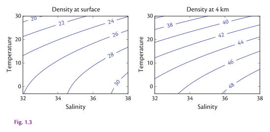
Dependence of density on temperature and salinity, and how it shifts with
pressure, is shown in Fig. 4.4.
Higher order equations of state are often used for higher accuracy, however
they’re out of scope for this course.
Figure 4.4.
Contours of density as a function of temperature and salinity for seawater. Contour labels are (density - 1000) kg m−3. In the interactive version, the slider sets the pressure from sea-level (p=105Pa, or 1000 mb) to 108Pa (about 10 km depth); the static fallback shows sea level and about 4 km depth. After Fig. 1.3 in AOFD (Vallis, 2017).
Like we did in the case of atmosphere, here we need to additional prognostic
equations, one of temperature and another for salinity:
∂t∂T+(u⋅∇)T=S˙T(4.57)
∂t∂S+(u⋅∇)S=S˙S(4.58)
where S˙T and S˙S are the sources and sinks of water temperature
and salinity, respectively.
Equations 4.48,
4.49,
4.56,
4.57, and
4.58 are the governing equations used in most
numerical ocean circulation models.
Nondimensionalization and scaling
A useful technique to simplify the analysis of the governing equations is to
scale the variables using characteristic values for each of the variables.
This is known as nondimensionalization
or scaling the equations.
In practice, for each (dependent or independent) variable x in the equations,
we define a characteristic value X.
For example, for the velocity u, we may pick the characteristic
value of U=1 m/s or U=10 m/s for the ocean or atmosphere, respectively.
We then divide each term in the equations by the characteristic value to
obtain a nondimensional (unitless) number.
This helps us identify the important parameters that govern the behavior of
the system and to group terms in the equations that are of similar magnitudes.
This is especially useful for large-scale flows, where the length and time
scales can vary over several orders of magnitude.
Let’s look, for example, at the vector equation for horizontal momentum
(thus, ignoring g for now):
∂t∂u+(u⋅∇)u=−ρ1∇p+ν∇2u(4.59)
The characteristic scales for each term are:
∂t∂u∼TU(4.60)
(u⋅∇)u∼LU2(4.61)
−ρ1∇p∼ρ1LP(4.62)
ν∇2u∼νL2U(4.63)
where U, T, L, and P are the characteristic scales for the velocity,
time, length, and pressure, respectively.
So, if for a given flow we can estimate these characteristic values, we can
easily determine which terms are important and which can be neglected.
This is the basis of scaling arguments in fluid mechanics.
This approach also enables characterizing the flows in terms of
nondimensional numbers.
For example, to describe how turbulent or laminar a flow is, it’s useful to
relate the inertial to the viscous terms in the momentum equation.
Their ratio is called the Reynolds number:
ν∇2u(u⋅∇)u∼L2νULU2=νUL≡Re(4.64)
You see that the Reynolds number is proportional to the velocity and length
scales each, and inversely proportional to the viscosity.
A larger Reynolds number corresponds to a more turbulent flow.
Exercises
Derive the Lagrangian form of the continuity equation from
the Eulerian form and vice versa. What is the key equation that relates the
two forms?
Consider two opposing, horizontal, surface currents along the x-axis.
In the vertical they uniformly span a mixed layer that extends from the
surface to the depth of 20 meters, with a magnitude of 1 m s−1.
The two currents meet at a stagnation zone that is 100 meters wide.
Calculate the downwelling velocity at the bottom of the mixed layer.
Assume ∇⋅u=0, no change in mean sea level, and no
flow in the y-direction.
Write out the Cauchy, Euler, and Navier-Stokes equations in vector form
and discuss their similarities and differences.
Give examples of flows that are well described by each of these equations.
Write a computer program that calculates the divergence of a second-order
tensor in a Cartesian, 3-dimensional coordinate system.
Write a function in your favorite programming language that takes a
value of temperature, salinity, and pressure and returns the density of
seawater. Assume linear dependence of density on temperature, salinity, and
pressure. Take the thermal expansion coefficient to be βT=1.67×10⁻⁴K−1,
the Haline contraction coefficient to be βS=7.8×10⁻⁴gkg−1,
and the compressibility coefficient to be βp=4.4×10⁻¹⁰Pa−1.
Take the reference density to be ρ0=1027kgm−3, the reference
temperature to be T0=283K, the reference salinity to be S0=35gkg−1,
and the reference pressure to be p0=105Pa.
When you implement your function, calculate the density of seawater for the
range of temperatures from -2 to 30 degrees Celsius, and salinities from 20 to
40 g/kg, and plot it as a contour plot as a function of temperature and salinity.
Make such plots for pressure values of 105, 106, and 107 Pa.
Calculate the Reynolds number for:
(a) a synoptic-scale mid-latitude cyclone in the atmosphere;
(b) an mesoscale ocean eddy;
(c) a river inflow into the ocean;
(d) a breaking ocean surface wave;
(e) water flowing through a pipe with a diameter of 0.1 m and flow speed of 1 m s−1.
Assume ν=10−5m2s−1 for air and ν=10−6m2s−1 for water.
Summary
In this chapter, we covered:
Conservation of mass (continuity equation) from both Eulerian and
Lagrangian perspectives;
Conservation of momentum equations: Cauchy, Euler, and Navier-Stokes;
The Reynolds number as a measure of the relative importance of inertial
to viscous forces in a flow;
The equation of state for seawater, relating density to temperature,
salinity, and pressure;
Examples of flows with different Reynolds numbers, from laminar pipe
flow to turbulent geophysical flows.
Chapter 5
Rotating flows
Fluids behave somewhat differently when in a rotating reference frame, for
example on the surface of a rotating planet while being observed from a fixed
location on that surface.
In this chapter we explore the effects of rotation on the flow.
We begin by deriving the temporal derivative of a general vector in a rotating
reference frame, and then apply it to find the velocity and acceleration in such
a frame.
From there we derive the centrifugal and Coriolis forces, and discuss their
implications for geophysical flows.
Rate of change of a rotating vector
Before determining what the velocity and acceleration should appear like
in a rotating reference frame (i.e. on the surface of a rotating planet), we
first need to understand how a vector that is fixed in the rotating frame
appears to change over time to the observer in the inertial (fixed) frame.
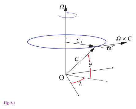
To do that, consider a vector C that rotates around an axis at a
constant angular velocity Ω (Fig. 5.1).
The angular velocity Ω is the rate of change of the angle in
the plane that is perpendicular to the axis of rotation, and is thus
dtdλ.
A unit vector m is oriented in the direction of the rate of change
of C, and is perpendicular to both C and Ω.
We will assume that Ω is constant.
This is a generally good assumption for the rotation rates of planets, at least
on time scales that we are interested in.
A small change in C can then be expressed as:
Figure 5.1.
A vector C rotating at an angular velocity Ω. It appears to be a constant vector in the rotating frame, whereas in the inertial frame it rotates according to (dC/dt)I=Ω×C. Drag the vector tips or use the controls to explore its perpendicular component, the angles θ and λ, and its tangent rate of change. After Fig. 2.1 in AOFD (Vallis, 2017).
δC=∣C∣cosθδλm(5.1)
The change in C is thus proportional to:
its magnitude;
the cosine of the angle between C and the horizontal plane
(i.e. the plane perpendicular to Ω);
the change in λ;
and, the unit vector m.
Notice now that using the definition of the cross product (Eq. 2.12),
and recalling that Ω=dtdλ,
we can write the change in C as:
δC=∣C∣∣Ω∣sin(π/2−θ)mδt=Ω×Cδt(5.2)
so the rate of change of a rotating vector, when observed from a fixed, inertial
frame is the cross product of the angular velocity and the vector itself:
(dtdC)I=Ω×C(5.3)
Going forward, we will use the subscript I to denote the inertial frame,
non-rotating reference frame.
Imagine now that you’re standing on top of the rotating vector C,
and are still relative to that rotating reference frame, much like standing
still on the surface of a rotating planet.
To you as the observer in the rotating frame, the vector C appears
to not change in any way.
Consider now another vector B that may change (in direction or
magnitude, or both) in the rotating reference frame.
We can then say that the rate of change of B in the inertial frame
is the vector sum of its two rates of change:
The rate of change of B in the rotating frame, and the rate of
change of the rotating frame itself:
(dtdB)I=(dtdB)R+Ω×B(5.4)
We now have a useful tool to use to determine the velocity and acceleration in
a rotating frame, such as that of of the surface of a rotating planet.
Velocity and acceleration in a rotating frame
Consider now a position vector r that locates a parcel in the rotating
frame.
The velocity of the parcel in the inertial frame is then given by the rate of
change of the position vector.
Apply Eq. 5.4 to r to get:
(dtdr)I=(dtdr)R+Ω×r(5.5)
As the time derivative of a position vector is velocity by definition, we can
write this as:
uI=uR+Ω×r(5.6)
This relates the inertial and rotating velocities.
Recall that we are interested in accelerations, as it’s the acceleration that
we solve for in the Navier-Stokes equations and relate to the forces that act
on the fluid.
We know that the acceleration is the rate of change of velocity, so let’s apply
Eq. 5.4 to the rotating velocity:
(dtduR)I=(dtduR)R+Ω×uR(5.7)
Now, use Eq. 5.6 to substitute for uI in
Eq. 5.7:
If Ω is constant, as we have assumed at the beginning,
inserting Eq. 5.10 into Eq.
5.9 yields:
(dtduI)I=(dtduR)R+2Ω×uR+Ω×Ω×r(5.11)
Since we’re interested in solving for the momentum in the rotating reference
(e.g., how windy will it be in my neighborhood tomorrow?), (dtduR)R
becomes our tendency of interest and the two new terms on the right-hand side
of Eq. 5.11 will appear as the new forces
of the momentum conservation balance (e.g., Navier-Stokes).
(dtduR)R, is the rate of change of
the relative velocity as observed in the rotating frame.
This is the rate of change of the velocity that you would measure with an
anemometer or current meter if position fixed relative to the rotating planet’s
surface.
(dtduI)I, is the rate of change of
the inertial velocity, i.e. the velocity as observed in the inertial
frame.
−2Ω×uR, is the
Coriolis acceleration
.
The Coriolis acceleration (and correspondingly, the Coriolis force) is
responsible for the organized rotation of large-scale atmospheric and oceanic
flows.
Notice that the Coriolis acceleration is always perpendicular to the relative
velocity uR.
This means that whenever we have a flow in a rotating frame, the Coriolis
force deflects the flow to the right or the left depending on the orientation
of Ω relative to the plane of the flow (i.e. the deflection is to the
right on the northern hemisphere and to the left on the southern hemisphere).
−Ω×Ω×r,
is the centrifugal acceleration.
It’s always antiparallel to the position vector r by definition.
Notice also that the centrifugal acceleration is not dependent on the velocity
of the parcel, but only on its position and the angular velocity of the
rotating frame.
This force could then be considered a body force, much like gravity.
Indeed, for practical reasons, centrifugal force if often bundled together
with gravitational force and expressed as a gradient of the scalar potential
Φ:
g−Ω×Ω×r≡−∇Φ(5.12)
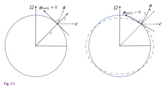
Effects of the centrifugal force on the effective gravity is illustrated
in Fig. 5.2.
If we bundle the centrifugal and the gravitational accelerations together and
express them as a geopotential gradient, we can write our momentum balance with
the effects of rotation as:
∂t∂u+(u⋅∇)u=−ρ1∇p−∇Φ−2Ω×u+ν∇2u(5.13)
Figure 5.2.
(a) Directions of forces and coordinates in true spherical geometry. g is the effective gravity (including the centrifugal force, C) and generally has a non-zero horizontal component. (b) A modified coordinate system, in which the upward vertical is opposite to g, so its horizontal component is identically zero. The dashed surface has constant geopotential. In the interactive, drag r to change latitude or drag Ω or C to change rotation strength; g0 denotes gravity without rotation. The differences between the radial and effective verticals, and between the sphere and the geopotential surface, are exaggerated and on Earth are similar to the thickness of the lines themselves. After Fig. 2.2 in AOFD (Vallis, 2017).
Coriolis force components
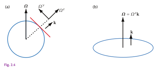
Figure 5.3.
(a) On the sphere the rotation vector Ω can be decomposed into two components, one in the local vertical and one along the local northward horizontal. That is, Ω=Ωyj+Ωzk where Ωy=Ωcosθ and Ωz=Ωsinθ. In geophysical fluid dynamics, the rotation vector in the local vertical is often the more important component in the horizontal momentum equations. On a rotating disk, (b), the rotation vector Ω is parallel to the local vertical k. Drag the position vector to vary latitude, including across the equator, or drag Ω to vary the angular speed. After Fig. 2.4 in AOFD (Vallis, 2017).
Let’s now examine in more detail the effects the Coriolis force on the flow.
The angular velocity Ω is a vector that points in the direction
oriented from the center of the Earth toward the North Pole
(see Fig. 5.3).
On the surface of the planet, thus, it has two components: A locally vertical
one, Ωz, and a meridional one, Ωy:
The Coriolis term thus contributes to all three components of the flow, and
their components vary with latitude.
Let’s look at the horizontal components first.
On geophysical scales, generally w≪u and so 2Ωwcosθ
can often be neglected.
The two dominant horizontal components of the Coriolis force then become
(−2Ωvsinθ,2Ωusinθ).
These components are zero at the Equator and increase poleward.
The vertical component, −2Ωucosθ, is negligible as well
compared to the other terms in the momentum equation, most notably the
gravitational acceleration g and the vertical pressure gradient that
balances it.
The horizontal effect is thus significantly more relevant for the horizontal
motion than the vertical one.
The practical implications of the Coriolis force on the flow is that it deflects
it toward the right on the Northern hemisphere and toward the left on the Southern
hemisphere.
If a parcel or a particle with some initial velocity on a rotating planet is
let undisturbed by other forces, it will appear to the observer standing on the
surface of the planet to move in circles with some radius.
We will calculate soon exactly how big this radius is depending on where on
the planet we are and the initial velocity of the parcel.
Let’s now incorporate the Coriolis force components into the vector-component
form of the momentum equation and apply some convenient approximations, namely
the f-plane and the β-plane approximations.
f-plane and β-plane approximations
Although geophysical fluids flow in a thin layer on a sphere, the curvature of
the surface of the planet is negligible for many applications.
Here we will make the so-called f-plane approximation in which the flow is
assumed to be on a flat plane tangent to the surface of a curved planet.
The main assumption of the f-plane approximation is that the planet’s rotation
exhibits only a locally vertical component anywhere on that planet’s surface.
In other words, we’ll neglect the horizontal component (i.e.Ωy).
With that assumption, the Coriolis force becomes strictly horizontal:
−2Ω×u=2Ωvsinθ−2Ωusinθ0(5.16)
Let’s now define the so-called Coriolis parameterf0=2Ωz=2Ωsinθ, so we can write the Coriolis force
more concisely as:
−f0k×u=f0v−f0u0(5.17)
The effect of the Coriolis force on the flow is now even more apparent:
A positive meridional flow causes a positive zonal acceleration,
and a positive zonal flow causes a negative meridional acceleration.
The implication of this is that the Coriolis force induces clockwise and
counterclockwise rotations in the Northern and Southern hemispheres,
respectively.
Ignoring viscosity for brevity, we can re-write our system of momentum equations as:
dtdu=−ρ1∂x∂p+f0v(5.18)
dtdv=−ρ1∂y∂p−f0u(5.19)
dtdw=−ρ1∂z∂p−g(5.20)
While on the small plane tangential to the planet’s surface the local rotation
may be uniform in space, in reality it does vary with latitude:
f=2Ωsinθ≈2Ωsinθ0+2Ω(θ−θ0)cosθ0(5.21)
for small deviations in θ.
We obtained this expression by expanding f in a Taylor series to the first
order around θ0.
On a plane, the above can be expressed as:
f=f0+βy(5.22)
where f0=2Ωsinθ0 and β=∂f/∂y=(2Ωcosθ0)/RE
(where RE is the radius of the Earth).
Geostrophic balance
Now that we have incorporated the effects of rotation into our equations of motion,
let’s evaluate the scales of the terms in the horizontal momentum equations.
We will start from Eq. 5.13, use the f-plane
notation for the Coriolis term, ignore the viscous terms, and drop the gravity
term as we’re looking at the flow in the horizontal plane:
∂t∂u+(u⋅∇)u+f×u=−ρ1∇p(5.23)
As we did in Section Nondimensionalization and scaling, let’s scale
each term on the left-hand side with their characteristic scales for mesoscale
ocean flow (L∼105m, T∼106s, U∼10−1m/s):
∂t∂u∼TU∼10−7
(u⋅∇)u∼LU2∼10−7
f×u∼f0U∼10−6
This means that on these oceanic scales (L∼100km, T∼1day),
the inertial terms are of the same order of magnitude as the Coriolis term.
In other words, rotation here is much more important than the local rate of
change or advection.
Also, whatever the scale of the pressure gradient term is, it is the only
term that can balance the rotation.
Thus, if we can state that the inertial terms can be neglected, we can also
state:
f×u≈−ρ1∇p(5.24)
or, in scalar component form:
fu≈−ρ1∂y∂p(5.25)
fv≈ρ1∂x∂p(5.26)
This balance is called the
geostrophic balance,
and it is a key concept in geophysical fluid dynamics.
It states that the flow is governed by the balance between the rotation and the
pressure gradient force.
Although the geostrophic balance is strictly an approximation and it never holds
exactly, large scale oceanic (L∼100km and larger) and atmospheric
(L∼1000km and larger) flows are often in geostrophic balance.
For the analysis of geophysical flows at such scales, it is then useful to
define the geostrophic velocity as:
ug=−ρf1∂y∂p(5.27)
vg=ρf1∂x∂p(5.28)
Notice that the geostrophic flow is always perpendicular to the pressure gradient,
which means it is parallel to the isobars (lines of constant pressure).
This also means that the isobars are streamlines of the geostrophic flow.
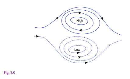
In the northern hemisphere (f>0), the geostrophic flow is cyclonic
(counter-clockwise) around the low-pressure region and anti-cyclonic
(clockwise) around the high-pressure region.
In the southern hemisphere (f<0), it is the opposite.
A nearly geostrophic flow is illustrated in Fig. 5.4.
Figure 5.4.
Geostrophic flow with a positive value of the Coriolis parameter f. Flow is parallel to the lines of constant pressure (isobars). Cyclonic flow is counterclockwise around a low pressure region and anticyclonic flow is clockwise around a high. If f were negative, as in the Southern Hemisphere, cyclonic flow would be clockwise and anticyclonic flow counterclockwise. In the interactive, the highs and lows are anomalies η in the height of the sea surface (ocean) or of a constant-pressure surface (atmosphere). Hydrostatic balance makes the horizontal pressure gradient ∇p=ρg∇η, so the geostrophic velocity is ug=(g/f)k×∇η. Drag, add, or remove highs and lows, set their amplitude and radius, and vary f (including its sign) and g. Color shows the geostrophic speed and particles drift with the flow. At the probe, the pressure gradient and Coriolis forces are equal and opposite, and the velocity is perpendicular to both. After Fig. 2.5 in AOFD (Vallis, 2017).
Rossby number
Recall that we required the inertial terms to be much smaller than the Coriolis
term for the geostrophic approximation to hold.
Like we did earlier with the Reynolds number to quantify how turbulent a flow is,
we can define the Rossby number as:
Although the Rossby number characterizes the relative importance of rotation in
the flow, notice that the rotation term is in the denominator.
The Rossby number is thus small for flows in which rotation dominates over
advection.
In general, flows with a Rossby number of 0.1 or smaller are considered
approximately geostrophically balanced.
Inertial oscillations
An analytical solution to the linearized horizontal momentum equations with
rotation gives rise to a steady circular motion called the inertial
oscillation.
Start from the linearized horizontal momentum equations with rotation
and with the pressure gradient force neglected:
∂t∂u+f×u=0(5.30)
In scalar component form, this is:
∂t∂u+fv=0(5.31)
∂t∂v−fu=0(5.32)
We are now looking for a solution for (u(t),v(t)).
These two equations are linear but coupled, so we need to decouple them
first to obtain the equations with one unknown variable each.
Differentiate each equation with respect to time to get:
∂t2∂2u+f∂t∂v=0(5.33)
∂t2∂2v−f∂t∂u=0(5.34)
and then insert Eqs. (5.31)-(5.32)
into the above to get:
∂t2∂2u+f2u=0(5.35)
∂t2∂2v+f2v=0(5.36)
The equations are now decoupled and each is a second-order, linear, homogeneous,
ordinary differential equation with constant coefficients.
The general solution to these equations is:
u=Acos(ft)+Bsin(ft)(5.37)
v=Ccos(ft)+Dsin(ft)(5.38)
To find the constants A, B, C, and D, take the initial conditions for
the velocity to be u(t=0)=[u0,v0].
This results in:
u=u0cos(ft)+v0sin(ft)(5.39)
v=v0cos(ft)−u0sin(ft)(5.40)
These equations describe a circular motion in the horizontal plane with a radius
of r0=u02+v02/f and a period of 2π/f.
It can be demonstrated that the motion is circular by integrating the velocities
(Eqs. 5.39-5.40) over time
to obtain displacements x(t) and y(t) and showing that the displacement
radius r=x2+y2 is constant, which can only be true for a circular
motion.
As the inertial oscillations scale with 1/f, they are larger and slower
near the Equator and smaller and faster near the poles.
For example, at 45 degrees latitude, f≈10−4s−1, and so the
period of the inertial oscillation is 2π/f≈17.5 hours.
Exercises
Calculate the effective gravity at the Earth’s Equator, poles, and 45 degrees
latitude, taking into effect centrifugal acceleration.
Using scale analysis, show that on geophysical scales the vertical
component of the Coriolis force is negligible compared to the other terms
in the momentum equation.
Show that the kinetic energy of an inertial oscillation is constant.
Summary
In this chapter, we covered:
The effects of rotation on fluid motion, including centrifugal and Coriolis
forces;
Derivation of velocity and acceleration in a rotating reference frame;
The Coriolis parameter f and its variation with latitude;
Inertial oscillations - circular motions that arise from the balance between
inertia and Coriolis force;
The solution for inertial oscillations showing circular motion with period
2π/f and radius r0=u02+v02/f.
Chapter 6
Stratified flows
Oceans and atmospheres are vertically stratified due to the effects of gravity.
In the previous chapters, we derived our equations for mass and momentum
conservation and we incorporated the effects of rotation.
We also explored how the density may vary in the vertical according to the
ideas gas law (in the atmosphere) or the equation of state for seawater.
We now explore the effects of density stratification on the flow and examine a
common approximation used for large-scale oceanic flows.
The Boussinesq equations
We will now explore within our framework the density perturbations that will
allow for buoyancy effects in a flow.
The Boussinesq approximation is an
approximation to the full equations of motion.
It assumes that the density and pressure perturbations are much smaller than
their means, and when applied to the Navier-Stokes equations, results in the
Boussinesq equations.
To start, we will allow the density to have small variations around its mean
value.
Decompose the density into the mean and the perturbation components:
ρ=ρ0+δρ(x,y,z,t)(6.1)
where ρ0 is the mean density and δρ is its perturbation.
Further, we decompose the pressure as:
p=p0(z)+δp(x,y,z,t)(6.2)
where p0 is the horizontally and temporally averaged pressure and δp
is its perturbation.
Unlike in the density decomposition, the mean pressure component is allowed to
vary in z.
For both quantities, we require that their perturbations are much smaller
than their respective means, i.e.δρ≪ρ0, δp≪p0.
In other words, the pressure vary much more in the vertical than in the
horizontal or over time, and any perturbations in density, including those in
the vertical, are much smaller than the mean density.
This approximation can be demonstrated to hold well by using the equation of
state for seawater (Eq. 4.56), for example.
The hydrostatic approximation in this framework is trivially satisfied:
dzdp0=−ρ0g(6.3)
Now that we’ve established the approximation we need, let’s proceed to apply it
to our momentum and continuity equations.
Momentum balance
Let’s first apply the Boussinesq approximation to the momentum balance.
Recall the Navier-Stokes equation with rotation
(Eq. 5.13), while neglecting the viscosity
term:
Now, recall that δρ≪ρ0, so we can drop the δρ
on the left-hand side:
ρ0(dtdu+f×u)=−∇δp+δρg(6.7)
dtdu+f×u=−ρ01∇δp+ρ0δρg(6.8)
For convenience of notation, let’s now define buoyancy
as b=−gδρ/ρ0, and re-write the above to obtain the
Boussinesq momentum equation:
dtdu+f×u=−ρ01∇δp+bk(6.9)
This equation states that now that we are in a gradually stratified fluid,
the gravity term is scaled by δρ/ρ0 to yield the appropriate
vertical acceleration, and the pressure gradient is due to the relatively
small perturbations in density δρ around the mean density ρ0.
Continuity
As we did for the momentum equation, we’ll now apply the Boussinesq approximation
(i.e.ρ=ρ0+δρ, δρ≪ρ0) to the
continuity equation.
Recall the continuity equation in its complete form:
Then, if we can state that that dδρ/dt≪ρ0∇⋅u,
which we will for the Boussinesq approximation, we recover the original
continuity equation for incompressible flows:
∇⋅u=0(6.12)
Note that we do not say that strictly dδρ/dt=0, but rather that
we can neglect it in this equation in favor of the velocity divergence term.
The evolution of δρ is still governed by the evolution of buoyancy,
which in turn is governed by the evolution of the temperature and salinity fields
and the equation of state.
The buoyancy b=−gδρ/ρ0 evolves as:
dtdb=b˙(6.13)
and the equation of state can be expressed in terms of buoyancy:
Finally the temperature and salinity evolve as before, following
Eqs. 4.57 and 4.58,
respectively.
Complete system of equations
The full system of Boussinesq equations for the ocean are then:
dtdu+f×u=−ρ01∇δp+bk(6.15)
∇⋅u=0(6.16)
dtdT=T˙(6.17)
dtdS=S˙(6.18)
b=b(T,S,p)(6.19)
Thermal wind balance
Now that we regard the ocean as a stratified and rotating fluid with a buoyancy
defined as b=−gδρ/ρ0, an emerging property of the flow
appears if we combine this fact with the geostrophic balance
(see Section Geostrophic balance).
Recall the components of geostrophic velocity (Eqs. 6.20-6.21):
Applying the hydrostatic approximation (Eq. 6.3)
to the above equations, and recalling the definition of buoyancy, we get:
∂z∂ug=−f1∂y∂b(6.24)
∂z∂vg=f1∂x∂b(6.25)
Equations 6.24-6.25 are known as the
thermal wind balance
(despite the name, it applies to oceans and atmopsheres alike!).
It states that the geostrophic velocity must be vertically sheared in the
presence of a horizontal buoyancy (density) gradient.
This is illustrated in Fig. 6.1.
Warm and light air means δρ<0 and thus b>0, while cold and dense
air means δρ>0 and thus b<0.
By hydrostasy, the vertical gradient of the pressure anomaly
∂δp/∂z is positive on the left and negative on the right.
This establishes negative horizontal pressure gradient aloft and a positive one
near the ground.
As the Coriolis force balances the horizontal pressure gradients, the geostrophic
wind is positive aloft (out of the page) and negative near the ground (into the page).
Thus, in a geostrophic balanced flow alone, introducing a horizontal buoyancy gradient
results in a vertical shear of the horizontal velocity.
Figure 6.1.
The mechanism of thermal wind. A cold fluid is denser than a warm fluid, so by hydrostasy the vertical pressure gradient is greater where the fluid is cold. Thus, pressure gradients form as shown, where “higher” and “lower” mean relative to the average at that height. The horizontal pressure gradients are balanced by the Coriolis force, producing (for f>0) the horizontal winds shown. Only the wind shear is given by the thermal wind. This is Fig. 2.6 in AOFD (Vallis, 2017).
Static instability
We now consider how a fluid parcel may oscillate when its density is perturbed
from its resting state and in absence of horizontal flow.
This allows us to study the vertical motions due to the vertical differences
in density and in isolation from other processes.
We will approach this problem by displacing a fluid parcel
adiabatically
(i.e. without exchange of heat or mass with the environment) by a small distance
δz and examining how the pressure and gravity forces act on it in response
(Fig. 6.2).
Recall that in Eq. 6.1 we allowed for the density
variations to be much smaller than the mean density, i.e.δρ≪ρ0.
Here we expand the density decomposition to a finer detail, specifically:
ρ=ρ0+ρ(z)+δρ(x,y,z,t)(6.26)
where we now differentiate between the mean density ρ0 and the
vertically-varying environmental density ρ(z), while the
perturbation δρ includes the vertical, horizontal, and temporal
density variations.
Figure 6.2.
A parcel is adiabatically displaced upward from level z to z+δz. A tilde denotes the value in the environment, and variables without tildes are those in the parcel. The parcel preserves its potential density, ρθ, which it takes from the environment at level z. If z+δz is the reference level, the potential density there is equal to the actual density. The parcel’s stability is determined by the difference between its density and the environmental density. If the difference is positive, the displacement is stable, and if negative the displacement is unstable. This is Fig. 2.8 in AOFD (Vallis, 2017).
As the fluid parcel is displaced adiabatically, its pressure changes
instantaneously to assume the same pressure as the environment.
However, its temperature and salinity do not change instantaneously, resulting
in a density change.
To account for the instantaneous change in pressure as the parcel is displaced
in height, rather than the actual density we need to consider the parcel’s
potential density, ρθ.
The potential density is the density the parcel would have if it were returned
to the level where the initial pressure was p0:
ρθ=ρ+cs2p0=ρ+cs2ρ0gz(6.27)
where cs2=∣∂p/∂ρ∣θ is the square of
the speed of sound in the fluid, which we here assume to be constant and equal
to ≈1500m/s.
cs2 is also related to the pressure compressibility of the fluid in the
equation of state for seawater (Eq. 4.56),
βp=1/(ρ0cs2).
Thus, if the parcel ascends or descends adiabatically, without a change in
temperature or salinity, but allowing it to assume environmental pressure,
its density will change but its potential density will remain constant.
Potential density is thus a useful concept for understanding the static stability
of the fluid.
Our goal now is to express a small change in density of the parcel relative to
the environment solely in terms of the vertical gradient of the potential density.
From Fig. 6.2, we start from:
δρ=ρ(z+δz)−ρ(z+δz)(6.28)
which is the difference between the parcel’s density and the environmental
density at the new level.
Taking the reference level to be z+δz means that:
ρ(z+δz)=ρθ(z+δz)(6.29)
so we can re-write the above as:
δρ=ρθ(z+δz)−ρθ(z+δz)(6.30)
Since the parcel’s potential density is conserved during the adiabatic
displacement, ρθ(z)=ρθ(z+δz), and recall that at
the starting level the parcel’s potential density equals the environmental
potential density, i.e.ρθ(z)=ρθ(z),
we can write:
δρ=ρθ(z)−ρθ(z+δz)(6.31)
Then, for small δz:
δρ=−∂z∂ρθδz(6.32)
The parcel’s static stability is thus determined by the vertical gradient of
the locally-referenced potential density of the environment,
ρθ:
∂z∂ρθ<0(statically stable)(6.33)
∂z∂ρθ>0(statically unstable)(6.34)
Now, to determine the oscillatory motion of the parcel, we apply Newton’s second
law and balance the acceleration of the parcel with the buoyancy force:
∂t2∂2δz=ρg(∂z∂ρθ)δz=−N2δz(6.35)
where we have defined the Brunt-Väisälä frequency
(or buoyancy frequency) as:
N2=−ρθg∂z∂ρθ=dzdb(6.36)
while noting that ρ(z)=ρθ(z) within
O(δz).
A parcel displaced from its equilibrium position will oscillate with angular
frequency N if N2>0 (statically stable), and freely accelerate
upward if N2<0 (statically unstable).
To demonstrate this, we recognize that, like the inertial oscillation
equations in Section Inertial oscillations, this is a second-order,
linear, homogeneous, ordinary differential equation with constant coefficients.
Its general solution is:
δz=Acos(Nt)+Bsin(Nt),if N2>0(6.37)
δz=Ce∣N∣t+De−∣N∣t,if N2<0(6.38)
As before, the values of coefficients A, B, C, and D can be found by
applying the initial conditions for δz and dδz/dt at t=0.
They are A=δzt=0, B=0, C=D=δzt=0/2, assuming
that the initial vertical velocity is zero.
In Python, the solution for the static instability oscillation can be coded
like this:
import numpy as npdef parcel_displacement(z0: float, N2: float, t: float) -> float: """Given initial parcel displacement z0, buoyancy frequency squared N2, return the parcel displacement at time t.""" N = np.sqrt(complex(N2)) if N2 > 0: # stable return z0 * np.cos(N * t) else: # unstable return z0 * np.cosh(np.abs(N) * t)
This oscillation is illustrated in Fig. 6.3.
In stable stratification (top panel), the parcel oscillates around its
equilibrium position with frequency N.
Higher stratification (larger N), leads to faster oscillations, while the
amplitude is controlled by the initial displacement δzt=0.
In unstable stratification (bottom panel), the parcel accelerates away from
its equilibrium position, with the rate of acceleration controlled by ∣N∣.
This solution is, of course, confined to the small values of δz.
This assumption is reasonable because the ocean is generally stably stratified,
and so large displacements, or large vertical extents of unstable stratification,
are uncommon.
Use the function above to calculate the trajectory of the parcel for different
values of N2 and initial displacement δzt=0, and get a sense of
how the oscillation changes with these parameters.
Figure 6.3.
Static instability oscillations in a stably (top) and unstably (bottom) stratified fluid.
Exercises
Use the linear equation of state for seawater to demonstrate that the
variations of density in the ocean are very small compared to the mean
density. How large (in percent relative change) are these variations with
respect to the changes in temperature, salinity, and pressure in the ocean?
Calculate the Brunt-Väisälä frequency for:
(a) a typical mid-latitude thermocline with temperature decreasing from 20°C
to 5°C over 500 m depth;
(b) the deep ocean where potential temperature decreases from 4°C to 2°C
over 2000 m depth.
Assume constant salinity of 35 g/kg.
Summary
In this chapter, we covered:
The Boussinesq approximation, which assumes density variations are small
compared to the mean density;
Decomposition of density and pressure into mean and perturbation components;
Static stability and its relationship to the vertical density gradient;
The Brunt-Väisälä frequency as a measure of stratification strength and
the natural frequency of vertical oscillations in a stratified fluid.
Chapter 7
Shallow water systems
In this chapter we move away from the continuously stratified ocean and
approximate it to a single layer of incompressible fluid that is also in
hydrostatic balance.
It turns out that this seemingly drastic approximation still allows the
reduced equation set to reproduce many observed large scale oceanic and
atmospheric phenomena.
In other words, the shallow water equations may be about the simplest equation
set thay yield relatively realistic and accurate atmospheric and oceanic flows.
The simplicity of these equations allow for easier interpretation and testing
of numerical implementations.
For this reasons, many high-end weather, ocean, and climate models begin with
a two-dimensional shallow water equations solver.
In fact, this system of equations is the basis for some operational
ocean prediction models, which are surprisingly accurate when applied to the
nearshore and coastal ocean.
We begin by introducing the key assumptions that allow the derivation of the
shallow water equations, and after that we derive the general solutions to the
equations.
Key assumptions
The name “shallow water” hints at the approximations that we will make about
the flow:
Shallow: The vertical scale of the flow is much smaller than the
horizontal scale. This doesn’t mean that there’s no vertical
flow, only that the horizontal flow is the dominant one (u,v≫w).
Water: The flow is incompressible (∇⋅u=0).
As a consequence, our flow is also hydrostatic (dp/dz=−ρg).
This approximation will show to be instrumental in allowing us to cast the
horizontal pressure gradient in terms of the surface elevation only.
The flow can then be seen as a thin layer of fluid over a rigid bottom
that may vary horizontally, and with a free surface that can freely
move in the vertical in response to the horizontal flow, bottom topography, and
incompressibility (Fig. 7.1).
This layer of fluid may or may not be covered on top by another layer of fluid,
with its own hydrostatic pressure imposed on the surface.
Figure 7.1.
A shallow water system. h is the thickness of a water column, H its mean thickness, η the height of the free surface and ηb is the height of the lower, rigid surface above some arbitrary origin, typically chosen such that the average of ηb is zero. Δη is the deviation free surface height, so we have η=ηb+h=H+Δη. This is Fig. 3.1 in AOFD (Vallis, 2017).
Shallow water equations
The shallow water equations consist of the momentum and the continuity
equations.
For 2-dimensional horizontal flow, the momentum equation can be expressed as
a single equation in vector form, or as two scalar equations in x and y.
Momentum equation
We begin from the vector momentum equation with rotation:
dtdu+f×u=−ρ1∇p+g(7.1)
In the vertical component of this equation we will neglect the vertical
acceleration to obtain the hydrostatic balance, as we did previously:
∂z∂p=−ρg(7.2)
We can integrate the hydrostatic balance in z to obtain the pressure as a
function of height:
∫p(z)pηdp=−∫zηρgdz(7.3)
where pη is the pressure at z=η.
As this is the pressure at the free surface, it corresponds to the atmospheric
pressure, if any.
Rearranging the terms after integration yields:
p(z)=pη+ρgη−ρgz(7.4)
We will now apply a horizontal gradient to both sides and assume for simplicity
that the horizontal gradient of pη is negligible compared to the other
terms.
In the context of the ocean surface, this would mean that the atmospheric
pressure varies in the horizontal much less than the water elevation.
This is almost always trivially satisfied.
Further, taking that neither the density nor gravity vary in the horizontal,
and noting that z as a vertical coordinate cannot vary in the horizontal,
we get:
∇p=ρg∇η(7.5)
Inserting Eq. 7.5 into
Eq. 7.1, and taking ∇ to be the horizontal
divergence going forward, we get:
dtdu+f×u=−g∇η(7.6)
which is the horizontal shallow water momentum equation with rotation.
Let’s now proceed to derive the shallow water continuity equation and complete
the system of equations.
Continuity equation
An intuitive approach to deriving the shallow water continuity is to consider
a column of fluid in a one-dimensional horizontal flow whose spatial variations
would cause a change in the surface elevation of that column due to the
incompressibility (Fig. 7.2).
Although the bottom surface here is shown to be flat, recall from Fig.
7.1 that it doesn’t need to be, and the water column height
h comprises of the mean water depth h (as measured from the rigid
bottom to the mean water level) plus the deviation of the free surface from the
mean water level, η:
h=h+η(7.7)
where the overline denotes a time average.
This implies η=0, by definition.
Figure 7.2.
The mass budget for a column of area A in a shallow water system. There is a non-zero vertical velocity at the top of the column if the mass convergence into the column is non-zero. This is Fig. 3.2 in AOFD (Vallis, 2017).
The difference between the amount of liquid flowing into and out of the column
thus must be balanced by a change in the surface elevation of the column:
u2h2−u1h1=∂t∂ηΔx(7.8)
Rearranging the terms leads to:
∂t∂η=Δxu2h2−u1h1≈∂x∂(uh)(7.9)
Generalized in vector form, this becomes the Eulerian form of the shallow water
continuity equation:
∂t∂η+∇⋅(hu)=0(7.10)
which states that the local change in surface elevation is governed by the
divergence of the horizontal flow through the water column.
Since a gradient of h can capture either the surface elevation or the mean
water depth gradients, this equation is valid for both flat and varying bottom
topography.
How about the Lagrangian form of the shallow water continuity?
From Eq. (7.10), expand the divergence term and
the water colum height h, and express the rate of change of η as a total
derivative to get:
dtdη−u⋅∇η+(h+η)∇⋅u+u⋅∇(h+η)=0(7.11)
dtdη+h∇⋅u+u⋅∇h=0(7.12)
Now, recognize that the advective component of the bottom topography gradient
u⋅∇h must be the Lagrangian rate of change of
the mean water depth, dh/dt, because the bottom topography is
fixed in time and the only way for a fluid parcel to experience a change in
mean water depth is to move horizontally.
Thus, we can write:
dtdη+h∇⋅u+dtdh=0(7.13)
or simply:
dtdh+h∇⋅u=0(7.14)
The Lagrangian form of the shallow water continuity can thus be expressed either
in terms of the total water column height h, in which case it takes the
familiar form, or in terms of the surface elevation η, in which case it
has an additional term that accounts for the bottom topography gradient.
To get the Eulerian form from here, we first need to recognize that
dη/dt=dh/dt because h=h+η, where h is the
mean water depth.
Then, expanding the Lagrangian derivative, we recover Eq.
7.10.
The complete equation set
The momentum and continuity equations that we derived above form the complete
set of shallow water equations.
In vector form, they are:
dtdu+f×u=−g∇η(7.15)
∂t∂η+∇⋅(hu)=0(7.16)
And in scalar form, in two dimensions:
∂t∂u+u∂x∂u+v∂y∂u−fv=−g∂x∂η(7.17)
∂t∂v+u∂x∂v+v∂y∂v+fu=−g∂y∂η(7.18)
∂t∂η+∂x∂(hu)+∂y∂(hv)=0(7.19)
which closes our system of equations.
In two dimensions, we thus have three equations for the three unknown
variables u, v, and η.
The flow is inviscid (no friction) but nonlinear (advective term
u⋅∇u is present), so this system of equations
allows for turbulence but does not dissipate energy.
Also, notice that the Coriolis force is present but has seamlessly percolated
from the starting equation without breaking any of the assumptions.
Thus, to consider shallow water systems in a non-rotating frame, simply drop
the Coriolis terms.
We now proceed to further simplify this equation set to derive a general
solution for the shallow water equations.
Poincaré waves
As we proceed to derive a solution to the equations
(7.17-7.19),
notice that the nonlinear terms get in the way of an analytical solution.
To work around this, we will assume a flat bottom H such that:
Although we do not require that the perturbations on their own
are small enough to neglect, the products of two perturbations are assumed to
be.
This allows us to linearize the equations and obtain:
∂t∂u+f×u+g∇η=0(7.23)
∂t∂η+H∇⋅u=0(7.24)
Or, in scalar form:
∂t∂u−fv+g∂x∂η=0(7.25)
∂t∂v+fu+g∂y∂η=0(7.26)
∂t∂η+H∂x∂u+H∂y∂v=0(7.27)
This is a linear system of three equations with three unknowns, u, v, and
η.
To solve it, we will look for wave-like solutions:
(u,v,η)=(u,v,η)ei(kx+ly−ωt)(7.28)
where u, v, and η are the wave amplitudes,
k and l are the zonal and meridional wavenumbers, respectively, and ω is the
angular frequency.
It is now worthwhile to pause and discuss what is a wave and how would we get
the idea to assume a wave form for the solution.
A wave is a disturbance in the medium that propagates through it with some
characteristic speed.
In our case, the wave is periodic, meaning that the disturbance repeats itself
in space and time.
That’s the meaning of the phase function ϕ=kx+ly−ωt in the
exponent: it determines where in the wave cycle we are at a given point in space
and time.
The assumption that the solution to the equations is a periodic wave is informed
by the fact that derivatives of periodic functions are also periodic, and
this will allow the wave form (eiϕ) to factor out of the equations, leaving
only the amplitudes and the wave parameters (k, l, ω) to
determine the solution.
Now, insert the wave form into Eqs. (7.25-7.27)
to get:
−iωu−fv+igkη=0(7.29)
−iωv+fu+iglη=0(7.30)
−iωη+iHku+iHlv=0(7.31)
or, in matrix form:
−iωfiHk−f−iωiHligkigl−iωuvη=0(7.32)
The solution to this system requires that the determinant of the matrix be zero,
which yields:
ω[ω2−f2−gH(k2+l2)]=0(7.33)
A trivial solution to this equation is ω=0, which corresponds to an
unperturbed, constant flow.
The other, non-trivial solution is the dispersion relation for shallow water
gravity waves in a rotating frame:
ω=f2+gH(k2+l2)(7.34)
This dispersion relationship connects the frequency to the wavenumber, and we
see that it scales with the Coriolis frequency f and the gravity wave
phase speed gH.
This general solution is called a Poincaré wave,
a surface gravity wave with effects of rotation.
Poincaré waves are also commonly referred to as
inertial-gravity waves.
Increasing the Coriolis parameter f while keeping the other parameters fixed
increases the frequency of the waves by enhancing the rotation.
Similarly, increasing the gravitational acceleration g or the mean water depth
H increases the frequency of the waves by enhancing the gravity wave phase
speed.
Notice also that the frequency ω scales linearly with the wavenumber
k2+l2, their ratio ω/(k2+l2) being the phase speed of the
wave:
cp=k2+l2ω=k2+l2f2+gH(7.35)
Figure 7.3.
Dispersion relation for Poincaré waves and non-rotating shallow water waves. Frequency is scaled by the Coriolis frequency f, and wavenumber by the inverse deformation radius gH/f. For small wavenumbers the frequency of the Poincaré waves is approximately f, and for high wavenumbers is asymptotes to that of non-rotating waves. This is Fig. 3.8 in AOFD (Vallis, 2017).
As there are two independent parameters in Eq. 7.34 that
originate from different terms in the shallow water equations, we can turn the
knobs on each to explore some limiting cases of the general solution.
Short gravity waves
In the case of short gravity waves, the pressure gradient terms (and thus,
gravity) dominate the Coriolis term (rotation):
gH(k2+l2)≫f2(7.36)
In this case, the dispersion relation simplifies to:
ω=gH(k2+l2)(7.37)
which is the dispersion relation for (non-rotating) shallow water gravity waves.
Notice, however, that we don’t require there to be no rotation at all to obtain
the non-rotating gravity waves.
Rather, we simply require that the waves are so short (high wavenumber) that the
Coriolis force is negligible compared to the gravity force.
The phase speed of these waves, that is, the speed at which they propagate, is:
Cp=kω=gh(7.38)
Real-life examples of this solution include tsunamis, wind-generated swell
waves on the ocean surface, or small ripples that propagate radially outward
when throwing a stone into a pond.
Inertial oscillations
If the wavenumber is so small (large wavelength) that the gravity term can be
neglected in favor of the Coriolis term, we recover a class of motion that we
explored earlier, the inertial oscillations.
In this case, the rotation dominates over the gravity:
f2≫gH(k2+l2)(7.39)
and the dispersion relation simplifies to:
ω=f(7.40)
which corresponds to a circular motion with the frequency that exactly equals
the Coriolis frequency (because (u,v)=(u,v)e−ift).
Recall that we already explored this solution by dropping the pressure gradient
terms in the rotating momentum equations back in Section
Inertial oscillations.
Here, it comes out as a limiting case from the general solution which we
couldn’t obtain prior to the shallow water approximations and linearization.
Kelvin waves
A special case of the general solution that is particularly relevant to the
atmospheric and oceanic dynamics is that of a linearized shallow water flow
that is bounded on one side by a solid boundary, such as a coastline.
The resulting solution is a special class of gravity waves called
Kelvin waves, which propagate as a shallow water
gravity wave along the solid boundary and whose propagation direction, as well
as the perturbation scale in the direction away from the boundary, are governed
by the planetary rotation rate.
Kelvin waves appear in both the atmosphere and the ocean.
To derive the Kelvin waves, we start from the linearized shallow water equations
(where we drop the primes for brevity):
∂t∂u−fv=−g∂x∂η(7.41)
∂t∂v+fu=−g∂y∂η(7.42)
∂t∂η+H(∂x∂u+∂y∂v)=0(7.43)
Now, suppose that our solid boundary is along the x-axis at y=0, which
allows us to neglect the meridional flow (v=0):
∂t∂u=−g∂x∂η(7.44)
fu=−g∂y∂η(7.45)
∂t∂η+H∂x∂u=0(7.46)
Differentiate Eq. 7.44 with respect to time and Eq. 7.46
with respect to x, and combine them to get:
∂t2∂2u−gH∂x2∂2u=0(7.47)
which is the standard wave equation, whose solution is a wave that propagates
with the phase speed c=gH.
We will thus assume a wave-like solution for u, like we did for the Poincaré
waves in Section Poincaré waves.
However, since we now have a solid boundary at y=0, we should also assume
that the solution should vary in the y direction (because it must be zero
at the boundary, and non-zero elsewhere).
The general solution for u may be:
u=u(y)ei(x−ct)(7.48)
Notice that we have now assumed the wave phase in the form of (x−ct),
as opposed to (kx−ωt).
This is because we already know the phase speed c, as well as for mathematical
convenience; the two wave forms are otherwise equivalent.
As for the elevation η, insert Eq. 7.48 into Eq.
7.46 to get:
η=gHu(y)ei(x−ct)(7.49)
We still need to solve for u(y), so we look for the equation that
has a derivative with respect to y.
So, insert Eqs. 7.48 and 7.49 into Eq.
7.45 to get:
fu(y)=−gH∂y∂u(y)(7.50)
which integrates to:
u(y)=u0e−gHfy=u0e−Ldy(7.51)
where
Ld=fgH(7.52)
is the Rossby radius of deformation
,
which is the length scale at which planetary rotation becomes important
relative to the effects of gravity (or buoyancy, in stratified flows).
The complete solutions for the shallow water Kelvin waves are then:
u=u0e−Ldyei(x−ct)(7.53)
η=gHu0e−Ldyei(x−ct)(7.54)
which is a wave in the direction along the rigid boundary (y=0) whose
amplitude decays exponentially away from the boundary, with a decay scale
equal to the Rossby radius of deformation Ld.
The choice of the orientation of the rigid boundary at y=0 is arbitrary;
if we had chosen the boundary at x=0, the solution would be a wave
propagating in the y direction and decaying in the x direction.
If it were oriented at some arbitrary angle between x and y axes, the
solution would be a 2-d wave in x and y and with their respective
wavenumbers controlling the phase speed in each direction.
Kelvin waves propagating eastward along the equator and decaying rapidly away to either side. This is Fig. 4.5 in Vallis (EAOD).
Conservative properties
We now look at some conservative properties of the shallow water equations,
namely the potential vorticity conservation and the conservation of energy.
The former is a material conservative property, meaning that it is conserved
along a fluid parcel as it moves and deforms.
The latter is a volume-integrated conservative property, meaning that it is
conserved in a control volume as the fluid evolves in time.
The conservation of potential vorticity yields some interesting emerging
properties of the flow, such as the vortex stretching due to the change in the
fluid depth, and the planetary waves due to the meridional variation of the
planetary vorticity (Coriolis parameter f).
Potential vorticity
Potential vorticity (PV) describes the rate
of rotation of a fluid parcel scaled by the fluid depth.
It is a material property, meaning that it is conserved along a fluid parcel
as it moves and deforms.
In shallow water systems, the conservation of potential vorticity allows us to
predict how an eddy’s spin may change as it moves into shallower or deeper water,
or if it moves north or south on a rotating planet.
First, some definitions as this is the first place that we encounter vorticity.
Vorticity is a measure of the local rotation of a fluid parcel,
and is defined as the curl of the velocity field:
In largely 2-d flows, the vertical component of vorticity is the most relevant,
and hereon we will use a separate symbol for it:
ζ=∂x∂v−∂y∂u(7.56)
Vorticity of a flow is a complementary property to its divergence.
A flow can be either rotational (non-zero vorticity) or irrotational
(zero vorticity), and either divergent (non-zero divergence) or non-divergent
(zero divergence).
It can be both rotational and divergent, or neither.
However, that they are complementary (and in a way, orthogonal) properties of
the flow can be shown mathematically by the fact that the divergence of
vorticity is always zero:
∇⋅∇×u=0(7.57)
This means simply that once you extract the vorticity from a flow by taking
∇×u, any divergence that may have been present in the
flow is left behind.
Back to our potential vorticity conservation derivation,
start from the momentum equation with effects of rotation:
∂t∂u+u⋅∇u+f×u=−g∇η(7.58)
We will rely on the following vector identity to rewrite the advective term:
u⋅∇u=21∇(u2)−u×(∇×u)(7.59)
and recognize ∇×u=ω as the vorticity
to rewrite the above as:
∂t∂u+(ω+f)×u=−g∇(η+21u2)(7.60)
Take a curl of this equation to get:
∂t∂(∇×u)+∇×[(ω+f)×u]=−g∇×∇(η+21u2)(7.61)
Since the curl of a gradient is always zero, the right-hand side vanishes, and
we are left with:
∂t∂ω+∇×[(ω+f)×u]=0(7.62)
Next, we use the vector triple product identity:
∇×ω×u=(u⋅∇)ω−(ω⋅∇)u+ω∇⋅u−u∇⋅ω(7.63)
Since vorticity must be divergence free (∇⋅ω=0),
and it’s perpendicular to the velocity vector (ω⋅u=0),
the second and the fourth terms vanish.
Define the vertical component of the vorticity to be:
where (ζ+f)/h is the potential vorticity,
and Eq. 7.70 is the conservation of potential
vorticity.
Let’s consider some implications of it.
First, without planetary rotation (f=0), potential vorticity is ζ/h.
Imagine a parcel of fluid with some vorticity ζ(for example, a small eddy).
The eddy propagates zonally over a seamount such that the mean water depth
gradually decreases.
As the eddy enters progressively shallower water, its vorticity must increase
so that the potential vorticity is conserved.
An cold eddy (with ζ>0) will thus rotate more rapidly (cyclonically, or
counter-clockwise in the Northern Hemisphere) as it approaches the tip of the
seamount where the water is shallowest, and then decrease again as it moves away
from the tip of the seamount into deeper water.
Similarly, a warm eddy (with ζ<0) will weaken its anticyclonic (clockwise)
rotation as it moves toward the tip of the seamount, and then strengthen it again
as it moves away from the tip of the seamount into deeper water.
Another consequence of the conservation of potential vorticity is that on a
β-plane, or more generally, a rotating sphere, where the Coriolis
parameter f varies with latitude, the vorticity of a parcel will adjust to
meridional displacements and changes in f to conserve potential vorticity.
The latter mechanism yields the so-called
Rossby waves, a key feature of mid-latitude weather
dynamics.
Energy
Start from the definitions of potential and kinetic energy:
PE=∫0hρgzdz=21ρgh2(7.71)
KE=∫0h21ρu2dz=21ρu2h(7.72)
The total energy is the sum of potential and kinetic energy:
E=PE+KE=21ρgh2+21ρu2h(7.73)
Let’s now proceed to derive the PE and KE equations for the shallow water
systems.
Recall the shallow water continuity equation:
dtdh+h∇⋅u=0(7.74)
Multiply it by gh to get:
dtd(2gh2)+gh2∇⋅u=0(7.75)
Expand the Lagrangian derivative:
∂t∂(2gh2)+u⋅∇(2gh2)+gh2∇⋅u=0(7.76)
Then, we borrow a half of the third term to combine it with the second term:
∂t∂(2gh2)+∇(u2gh2)+2gh2∇⋅u=0(7.77)
which is the equation for the evolution of potential energy.
Note that the density ρ is assumed constant and is omitted here for brevity.
Next, recall the momentum equation, assuming uniform mean water depth for
simplicity:
dtdu=−g∇h(7.78)
Multiply this by u and re-arrange to get:
uhdtdu+guh∇h=0(7.79)
dtd(2hu2)−2u2dtdh+gu∇(2h2)=0(7.80)
Recall the shallow water continuity to write:
dtd(2hu2)+2hu2∇⋅u+gu∇(2h2)=0(7.81)
Expand the Lagrangian derivative:
∂t∂(2hu2)+u⋅∇(2hu2)+2hu2∇⋅u+gu∇(2h2)=0(7.82)
and combine the second and third terms to write:
∂t∂(2hu2)+∇⋅(u2hu2)+gu∇(2h2)=0(7.83)
which is the equation for the evolution of kinetic energy.
which is the conservation of total energy E=PE+KE, and
F=u(21hu2+gh2) is the energy flux
such that we can write:
∂t∂E+∇⋅F=0(7.85)
The total energy of the system E is thus conserved and entirely governed by
the divergence of the energy flux F.
Rossby waves
One emerging pattern from the conservation of potential vorticity arises if
the planetary vorticity f is allowed to vary with latitude.
This is true on a sphere where f=2Ωsin(θ), or on a β-plane
where f=f0+βy.
This pattern is called Rossby waves (also called
planetary waves) and is among the most important
classes of motions in both the ocean and the atmosphere.
To derive the solution for Rossby waves, we start from the shallow-water potential
vorticity conservation equation:
dtd(hζ+f)=0(7.86)
To simplify the derivation, we will assume a flat bottom so that
dtd(ζ+f)=0(7.87)
Expand the Lagrangian derivative to get:
∂t∂ζ+u⋅∇ζ+vβ=0(7.88)
which is the potential vorticity conservation equation on a β-plane.
We still have only one equation with two unknowns, albeit two related unknowns
(relative vorticity ζ and velocity u).
We somehow need to reduce them to one unknown variable.
One approach is to introduce a streamfunctionψ such that:
(u,v)=(−∂y∂ψ,∂x∂ψ)(7.89)
We can then express the relative vorticity in terms of the streamfunction as:
ζ=∂x∂v−∂y∂u=∂x2∂2ψ+∂y2∂2ψ=∇2ψ(7.90)
Then, insert Eqs. 7.89 and 7.90
into Eq. 7.88, and linearize u in the
advective term such that the relative vorticity is only advected by the steady
zonal flow U:
∂t∂∇2ψ+U∂x∂∇2ψ+β∂x∂ψ=0(7.91)
which is the potential vorticity equation on a β-plane in terms of the
streamfunction.
As before, assume a wave-like solution but this time for the streamfunction:
As before, k=0 is a trivial and non-interesting solution, as it corresponds
to there being no wave at all.
For the non-trivial solution, rearranging the terms to get the equation for
frequency yields the dispersion relation for Rossby waves:
ω=Uk−kβ(7.94)
The phase speed of Rossby waves is:
cp=kω=U−k2β(7.95)
and their group speed, that is, the speed at which the wave energy propagates,
is:
cg=∂k∂ω=U+k2β(7.96)
Like in the case of the Poincaré waves, the frequency (or the phase speed) of
Rossby waves do not depend on the wave amplitude (ψ), which is a
consequence of the linearization.
Instead, they depend on the wavenumber k (inverse wave length), the magnitude
of the steady zonal flow U, and the meridional Coriolis gradient β.
U is here simply a linear Doppler shift term, and does not affect the
wave’s intrinsic properties; it merely translates it.
The second term, −β/k, is the intrinsic frequency of Rossby waves,
which is always negative because β=2Ωcosθ>0.
This means that Rossby waves always propagate westward relative to the mean flow
(cp−U<0).
Further, depending on their scale and the magnitude of the zonal flow, their
phase can be stationary (cp=0) or even eastward propagating (cp>0).
However, their intrinsic group speed is always positive (cg>0), and thus,
even in the case of no background zonal flow (U=0), their energy propagates
eastward.
Figure 7.5.
A two-dimensional (x-y) Rossby wave. An initial disturbance displaces a material line at constant latitude (the straight horizontal line) to the solid line marked η(t=0). Conservation of potential vorticity, ζ+βy, leads to the production of relative vorticity, ζ, as shown. The associated velocity field (arrows on the circles) then advects the fluid parcels, and the material line evolves into the dashed line with the phase propagating westward. This is Fig. 6.3 in Vallis (EAOD).
Rossby waves are named after Carl-Gustaf Rossby, an American meteorologist of
Swedish origin, who first identified these waves while studying large scale
flow in the atmosphere in the 1930s.
The Carl-Gustaf Rossby Research Medal is the highest award in atmospheric
sciences, has been awarded by the American Meteorological Society since 1951.
Exercises
Assuming shallow water approximation and mid-latitudes, quantify the
relative importance of planetary rotation in the flow for (a) wind-generated
swell waves, (b) a submesoscale eddy, (c) Gulf Stream, and (d) a synoptic-scale
cyclone in the atmosphere.
Consider characteristic mid-latitude flows on Earth, Jupiter, and Titan.
At what spatial scales does the gravity play equal role as the rotation?
Assume the shallow water dispersion relationship for your analysis.
An ocean eddy with initial relative vorticity ζ0 begins its
journey northward at 30∘N and depth of 2000 m and travels with the
mean flow to 40∘N and depth of 1000 m.
Assuming the potential vorticity of the eddy is conserved, calculate the its
final relative vorticity.
Find the expression for the wavenumber of a stationary Rossby wave as
a function of latitude and the mean zonal flow. Then, calculate the wavelength
of a stationary Rossby wave at 45∘N, in a mean zonal flow of 10 m/s.
Summary
In this chapter, we covered:
The shallow water equations as a simplified model for large-scale ocean and atmospheric flows;
Key assumptions of the shallow water system: horizontal scales much larger than vertical scales, incompressible flow, and hydrostatic balance;
Conservation of potential vorticity and its role in generating relative vorticity as fluid parcels move meridionally.
Rossby waves - westward propagating planetary waves that arise from the variation of the Coriolis parameter with latitude;
The dispersion relationship and phase speed of Rossby waves;
Chapter 8
Turbulence
Turbulence is the nonlinear and chaotic fluid motion that occurs when a fluid
is driven by sufficiently strong forces.
It is characterized by large fluctuations in time and space and over a broad
range of scales.
Fluid elements with high vorticity of either sign move and interact with each
other, transferring energy and vorticity across scales.
In this chapter, we investigate turbulence from the point of view of the
governing equations of fluid motion.
The key pursuit of fluid mechanics of turbulence is to predict the evolution of
mean flow while accounting for the effects of turbulence.
We begin by introducing the Reynolds decomposition, a fundamental
tool in the study of turbulence that allows separating the flow into a slowly
evolving mean part and a rapidly fluctuating turbulent part.
Applying the Reynolds decomposition to the Navier-Stokes equation leads to the
Reynolds-averaged Navier-Stokes (RANS) equation, which is the prognostic
equation for the mean flow.
We will discuss the so-called closure problem of turbulence, which is the
challenge of representing the effects of the smallest scales on the larger scales.
Using the RANS equation, we will derive the turbulent kinetic energy budget
equation, and investigate the turbulent cascade in both 2D and 3D flows.
The new understanding from this chapter will allow us to study the boundary
layers in the atmosphere and the ocean alike.
Reynolds decomposition
Before we apply any scale separation to the Navier-Stokes equation, let’s
first define the Reynolds decomposition that breaks the flow u into the
time-mean and fluctuating parts:
u(x,t)=u(x)+u′(x,t)(8.1)
The time average is defined as:
u(x)=T1∫t0t0+Tu(x,t)dt(8.2)
Already we need to make a choice about the averaging time T.
This choice is arbitrary and usually driven by the practical limitations of the
problem.
Typical weather and ocean ciculation models take T to be on the order of
seconds (for a regional weather prediction model) to minutes
(for a mesoscale ocean circulation model).
The turbulence itself operates on much shorter time scales, typically on the
order of milliseconds to seconds for atmospheric and oceanic flows.
Let’s look at some mathematical properties of the Reynolds decomposition.
If we take the time average of 8.1, we get:
u(x,t)=u(x)+u′(x,t)(8.3)
which leads to:
u′(x,t)=0(8.4)
Notice that we specifically average over time, not space, which allows the mean
flow to vary in space.
We could have as easily defined the average in 8.1
to be over a spatial domain (or any other dimension), and those are indeed
useful for other things.
Figure 8.1.
An 10-second example sequence of horizontal velocity u (blue) measured at 1000 Hz using a Constant Temperature Anemometer in the Air-Sea Interaction Saltwater Tank (ASIST) at the University of Miami. Dashed black line shows the time-mean velocity u calculated over the 10-second interval, and the orange line shows the fluctuating part.
The averaging operation is commutative with respect to derivatives and integrals,
over space or time alike:
∂t∂u=∂t∂u(8.5)
∇⋅u=∇⋅u(8.6)
∫udt=∫udt(8.7)
Although here we have defined the Reynolds decomposition using the velocity
field, it can be applied to any field variable, vector or scalar alike.
If the flow is incompressible (∇⋅u=0), then the mean
flow is incompressible as well:
∇⋅u=0(8.8)
and by definition the fluctuating field must also be divergence-free:
∇⋅u=∇⋅(u+u′)=∇⋅u+∇⋅u′=0(8.9)
∇⋅u′=0(8.10)
An example of the Reynolds decomposition applied to a measured turbulent velocity
time series is shown in Fig. 8.1.
Reynolds-Averaged Navier-Stokes (RANS) equation
We seek the governing equations for the mean flow that include the effects of
the fluctuating field (turbulence).
To do that, let’s apply the Reynolds decomposition to the Navier-Stokes equation
and take the time average of the resulting equation.
We begin by writing out Eq. 4.40 without the
body forces, for simplicity (as the body forces won’t be affected by the
Reynolds decomposition):
∂t∂u+u⋅∇u=−ρ1∇p+ν∇2u(8.11)
It’s at this time useful to re-cast this equation in the momentum-conservative
form that is prognostic for the momentum ρu rather than just the
velocity u.
To do that, multiply Eq. 8.11 by ρ to get:
ρ∂t∂u+ρu⋅∇u=−∇p+μ∇2u(8.12)
while recalling that the kinematic viscosity ν is defined as
ν=μ/ρ.
Now, we will use the Eulerian form of the continuity equation
(Eq. 4.4) to reframe the left-hand side of Eq.
8.12 in terms of the momentum ρu:
Take a moment to notice and understand that uu in the last
term is a second-order tensor rather than a scalar
u⋅u=u2.
Its physical interpretation as advective flux still remains as before; the only
difference is that the advective velocity is now inside the derivative.
Back to our momentum equation (Eq. 8.12), we can now write it as:
∂t∂(ρu)+∇⋅(ρuu)=−∇p+μ∇2u(8.14)
and in case of incompressible flows (∇⋅u=0):
∂t∂u+∇⋅(uu)=−ρ1∇p+ν∇2u(8.15)
As we haven’t applied the Reynolds decomposition yet, we are still describing
the full flow with all its turbulent fluctuations.
Remember that we are interested in the solution for the mean flow that accounts
for the effects of turbulence, so we need apply the Reynolds decomposition to
u and p, time average the resulting equation, and notice that
u′ and p′ are both zero:
which is the Reynolds-Averaged Navier-Stokes (RANS) equation
.
The term u′u′ is called the
Reynolds stress tensor
and ∇⋅(u′u′) is the
Reynolds stress divergence.
As this term is the only one that features the velocity fluctuations, it must
be the contribution of turbulence to the mean flow!
The Reynolds-averaged continuity equation is much simpler to derive and is
just:
∇⋅u=0(8.20)
Between Eqs. 8.19 and 8.20 we have
two equations with three unknowns: u, p, and
u′u′.
To close the system, we need to find an equation for the Reynolds stress tensor,
which brings us to the infamous closure problem of turbulence.
Closure problem
The closure problem of turbulence arose as a key obstacle in the theoretical
study of turbulence based on the Navier-Stokes equation.
To illustrate it, try to derive the equation for the evolution of the Reynolds
stress u′u′.
Suppose that the Reynolds stress evolves according to the yet to be determined
sources and sinks of the Reynolds stress:
dtd(u′u′)=sources−sinks(8.21)
Expanding the time derivative in a momentum-conservative form and time averaging
yields an equation similar to Eq. 8.18:
dtd(u′u′)=∂t∂(u′u′)+∇⋅(uu′u′)+∇⋅(u′u′u′)(8.22)
See, if we try to find the equation for the evolution of the Reynolds stress,
we end up with the flux of the flux itself as a new unknown.
Further, if we tried to seek the equation for this new cubic term, we would
end up with an equation that includes a quartic term of u′:
Then, if we tried to find the equation for the quartic term, we would end up
with a quintic term, and so on in an infinitely recursive pursuit.
The fact that we cannot close the RANS equations unless we somehow approximate
the Reynolds stress tensor is known as the closure problem of turbulence.
On one hand, it’s relieving that we don’t have to figure out the sources and
sinks for the Reynolds stress tensor in Eq. (8.21).
On the other hand, we still need to come up with some model or approximation
for the Reynolds stress tensor to solve the RANS equations.
Decades of theoretical, experimental, and numerical research have been devoted
to exactly this question: how to approximate u′u′
in terms of the mean flow u and its gradients.
Reynolds stress
Recall from Chapter Conservation of mass and momentum where we first derived the
Cauchy momentum equation (Eq. 4.23), ignoring the body forces
for brevity:
where we had described the stress tensor σ as a combination
of the normal stresses (pressure) on the diagonal and the deviatoric stresses
off the diagonal:
Then, in Section Viscous forces, we stated that for a Newtonian fluid
the deviatoric stresses can be approximated with the velocity gradients, an
approximation that was established in the laboratory:
∇⋅τ=ν∇2u(8.27)
Now, in addition to the viscous stresses, we have the turbulent Reynolds stresses
introduced in Eq. 8.19.
The turbulent Reynolds stresses arise due to the scale separation between the
large-scale mean flow and the turbulent fluctuations, which we introduced when
we applied the Reynolds decomposition to the velocity field.
Eq. 8.19 can be rewritten more concisely by applying the divergence
operator to the pressure and Reynolds and viscous stresses as a whole:
∂t∂u+∇⋅(uu)=ρ1∇⋅(μ∇⋅u−p−ρu′u′)(8.28)
If it’s not obvious already, notice that ρu′u′
is the only term that makes Eq. 8.28 different from the
original Navier-Stokes equation Eq. 8.15.
Thus, if we apply a scale separation (i.e. the Reynolds decomposition)
to the velocity field such that we distinguish between the mean flow and the
fluctuations, the equation for the mean flow contains an additional term that
quantifies the contribution of the turbulent fluctuations to the mean.
Note that, strictly speaking, ρu′u′ is a
stress (as in, momentum flux), however it’s common to refer to
u′u′ as the Reynolds stress as well, even when
the density is omitted.
Let’s look at this Reynolds stress tensor in more detail.
Using our usual notation for the velocity vector to be u=(u,v,w),
the components of the Reynolds stress tensor are:
The diagonal components of this tensor (u′u′, v′v′, and
w′w′) are called the normal stresses, and the off-diagonal
components (u′v′, u′w′, v′w′) are called
the shear stresses.
The Reynolds stress tensor is symmetric, which means that
u′v′=v′u′, u′w′=w′u′, and
v′w′=w′v′.
It is only the shear stresses that contribute to the turbulent transport of
momentum.
An important property of boundary layer physics, the
Turbulent Kinetic Energy (TKE) is half
the sum of the diagonal components of the Reynolds stress tensor:
k=21(u′u′+v′v′+w′w′)(8.30)
From the point of view of the Reynolds decomposition into the mean and
fluctuations from the mean, TKE is the sum of velocity variances.
TKE plays an important role in parameterizing the subgrid-scale turbulent
processes in the boundary layer components of weather and ocean prediction
models.
u′w′ and v′w′ are also very important quantities in
the study of air-sea interaction, as they govern the momentum exchange between
the atmospheric surface layer, the ocean surface waves, and the upper-ocean
boundary layer.
In numerical models, the vector equations must be written out explicitly in
scalar component form (remember that computers only deal with numbers and never
with higher level concepts like orientation or vectors).
It’s thus a useful exercise to write out the RANS equation
(Eq. 8.28) as a system of scalar equations, one for each
component of the mean velocity vector:
Via the finite difference, finite volume, or finite element methods, each term
in these equations can be written out using simple arithmetic expressions,
and most numerical flow prediction models do exactly that.
Turbulent kinetic energy budget
Turbulent kinetic energy (TKE) is a fundamental quantity in the study of
turbulence.
It’s a prognostic variable in many subgrid-scale parametric models of
atmospheric and oceanic boundary layers.
Here we derive the prognostic equation for TKE from the fundamental equations
with Reynolds decomposition, often referred to as the TKE budget equation.
The derivation of the TKE budget equation involves the following steps:
Start from the Navier-Stokes equation (Eq. 8.11)
and apply the Reynolds decomposition to the velocity field.
Subtract the RANS equation from the original Navier-Stokes equation
with Reynolds decomposition to obtain the equation for the velocity
fluctuations.
Multiply the equation for the velocity fluctuations by the fluctuating
velocity components and time-average to obtain the equation for the TKE.
For completeness, we will also consider the buoyancy term that we derived in
the Boussinesq approximation, as it will turn out that this term plays a role
in the TKE budget.
We start from the Navier-Stokes equation but in the advective (non-conservative)
form, rather than the flux (conservative) form, as the advective form makes the
TKE budget derivation more straightforward (they are equivalent for
incompressible flows, ∇⋅u=0).
∂t∂u+(u⋅∇)u=−ρ1∇p+ρδρg+ν∇2u(8.34)
Apply the Reynolds decomposition to u, p, and δρ to get:
Finally, time-average to get the TKE budget equation, noting that the last term
on the left-hand side drops out due to time-averaging, and that
k≡21u′2:
So far we broke down the advective term from the original Navier-Stokes equation
to produce three new terms.
We’re still left with the viscous term, which can be rearranged into two terms
for a more intuitive physical interpretation.
Here we’ll use the following identity to expand the Laplacian:
Let’s look at each term in Eq. (8.42) and discuss its
physical meaning:
∂t∂k: Eulerian rate of change of TKE in
a fixed point in space.
u⋅∇k: Advection of TKE by the mean
flow. Like any other fluid property, TKE as well is subject to advection by
the mean flow, i.e.dk/dt=∂k/∂t+u⋅∇k.
−21∇⋅(u′u′u′)
is the turbulent transport of TKE. In other words, this term quantifies how
much turbulent eddies are transported by the turbulent eddies themselves.
−(u′u′⋅∇)u is the
production of TKE by the mean flow, also known as the shear production.
−ρ1u′∇p′ is the
production of TKE by the turbulent fluctuations of the pressure gradient,
also known as pressure diffusion.
ρδρ′u′⋅g
is the production of TKE by buoyancy. Notice the dot product between the
velocity vector and the gravitational acceleration, which means that the
buoyancy production occurs only by the vertical velocity component, and is
scaled by the buoyancy anomaly δρ′. The stronger the stratification
of the fluid, the larger the buoyancy production (or dissipation, depending on
the sign of stratification) of TKE.
Of course, this term is non-negligible only in the vertical direction.
ν∇2k is the dissipation of TKE by molecular diffusion,
analogous to the viscous diffusion of momentum in the original Navier-Stokes
equation.
−ν∇u′⋅∇u′ is the
turbulent eddy dissipation of TKE. Note that ∇u′ are rank-2
tensors, so the inner product ∇u′⋅∇u′
through double contraction results in a scalar.
In atmospheric and oceanic boundary layer modeling, the TKE budget equation
(Eq. 8.42) is often simplified by assuming stationarity and
horizontal homogeneity, and applying it to the vertical direction near the
boundary.
A simpler budget is then found to be the balance between shear and buoyancy
production of TKE and its dissipation by eddy viscosity, respectively:
−u′w′∂z∂u+w′b′−ν[(∂z∂u′)2+(∂z∂w′)2]=0(8.43)
Given Eq. 8.42 and the interpretation of its terms,
we can proceed to apply dimensional analysis in an attempt to learn the
distribution and transfer of turbulence across spatial scales.
Turbulent cascade
The two most common sources of turbulence are shear (mechanical) and buoyancy
(thermodynamic).
As such, the turbulent energy is predominantly generated at the larger scales,
where the largest coherent eddies tend to be of the same scale as the flow
itself.
For example, the largest eddies that the Gulf Stream sheds are of similar
diameter as the width of the Gulf Stream itself.
Similarly, the largest eddies in a coffee cup are of similar size as the spoon
that does the stirring.
An example of buoyancy generation of turbulence is the convection in the
atmospheric boundary layer due to cool air over warm land or ocean surface.
So, most turbulence tends to be produced at the scales many orders of magnitude
that of the viscous scales.
At the smallest scales, we know that viscosity does the work to dissipate
mechanical energy into heat.
What happens between the largest and the smallest scales is less clear and is
the subject of this section.
A concept of turbulent energy cascade,
first introduced by Richardson (1920),
suggests that the energy is transferred from the large to the small scales,
and that this transfer is a cascade.
He put it succinctly as:
Big whirls have little whirls,
Which feed on their velocity;And little whirls have lesser whirls,And so on to viscosity.
To answer how the velocity statistics are distributed from the largest to the
smallest scales, we evaluate the TKE budget equation for a very turbulent flow
in which Re=UL/ν is very large.
The turbulent cascade is illustrated in Fig. 8.2.
Figure 8.2.
The passage of energy to smaller scales: eddies at large scale break up into ones at smaller scale, thereby transferring energy to smaller scales. The eddies in reality are embedded within each other. If the passage occurs between eddies of similar sizes (i.e., if it is spectrally local), the transfer is said to be a cascade. This is Figure 11.2 from Vallis (AOFD).
We may first ask at what length scale does the viscosity become a dominant
player.
As useful tools we will recall dimensional analysis and the Reynolds number,
which quantified the relative importance of inertial over viscous forces.
Re=νUL(8.44)
If we know that at the largest (think, geophysical) scales the viscosity is
negligible (large Re), we could say that the viscosity becomes more important
than turbulent motion at the scale at which Re≈1.
From there, we can define the viscous length scale as:
Lν=Uν(8.45)
What are some characteristic values of Lν in the ocean and in the atmosphere?
An ocean flow with U≈10−1 m/s and viscosity of ν≈10−6 m2/s
gives Lν≈10−5 m, or, one hundredth of a millimeter.
In the atmosphere with U≈10 m/s and viscosity of ν≈10−5 m2/s,
we get Lν≈10−6 m, or, one micron.
These are obviously very small scales.
Kolmogorov’s hypotheses and scales
To answer what happens to the flow statistics between the largest scales at
which the turbulence is generated and the smallest scales at which viscosity
dissipates all mechanical energy into heat, Kolmogorov (1941) proposed
a new theory of turbulence based on three hypotheses.
Kolmogorov’s three turbulence hypotheses are:
Hypothesis of local isotropy: At sufficiently high Re and
sufficiently small L, the turbulence is locally isotropic,
i.e. the flow statistics at a point are the same in all directions.
In other words, the small-scale turbulence is homogeneous and has no preferred
direction.
First similarity hypothesis: At sufficiently high Re and
sufficiently small L, the flow statistics have a universal form
that is uniquely determined by the viscosity ν and the energy dissipation
rate ε.
In other words, small-scale turbulence is independent of the large-scale flow
features such as the geometry and boundary conditions.
Second similarity hypothesis: At sufficiently high Re and
and sufficiently large L, the flow statistics have a universal form
that is uniquely determined by the energy dissipation rate ε,
and that is independent of viscosity ν.
In other words, large-scale turbulence is governed by turbulent eddy dissipation
and is independent of molecular viscosity.
The energy dissipation rate ε comes straight from the TKE budget
equation (8.42) and is defined as:
ε=ν∇u′⋅∇u′(8.46)
In a nutshell, Kolmogorov’s three hypotheses state that a turbulent flow at
sufficiently small scales is the same looking in all directions, that
statistically all such turbulent flows are the same, and that they are uniquely
determined by either by energy dissipation rate alone, or by the energy
dissipation rate and viscosity, depending on the scale.
Through dimensional analysis, Kolmogorov also introduced three fundamental
turbulent scales, now commonly known as Kolmogorov scales:
The Kolmogorov length scale ηk, the velocity scale uη, and the time
scale τη.
Let’s use dimensional analysis to determine the length scale ηk.
Following Kolmogorov’s first similarity hypothesis, we assume that ηk is a
function of only ν and ε:
ηk=f(ν,ε)=νaεb(8.47)
The powers a and b can be determined by matching the dimensions on both sides:
L=(L2T−1)a(L2T−3)b(8.48)
which leads to:
1=2a+2b(8.49)
0=−a−3b(8.50)
so we arrive at a=3/4 and b=−1/4, giving us the Kolmogorov length scale:
ηk=(εν3)1/4(8.51)
This is the scale at which the energy dissipation by molecular diffusion
balances the energy input by the mean flow.
(The subscript k stands for “Kolmogorov”, and although it is not commonly used
in the literature, here I use it to avoid a notion conflict with η used
for surface elevation.)
Following the same approach, we can derive the Kolmogorov time scale:
τη=(εν)1/2(8.52)
which is the time scale at which the smallest coherent eddy can exist.
Finally, the Kolmogorov velocity scale is:
uη=(εν)1/4(8.53)
Any flow feature at scales smaller than these is governed by viscous dissipation
of kinetic energy into heat.
Examining the Reynolds number using the Kolmogorov scales indeed shows that
it reduces to unity, consistent with Eq. 8.45:
Reη=νuηη=ν(εν)1/4(ν3/ε)1/4=1(8.54)
Figure 8.3.
The energy spectrum in three-dimensional turbulence, in the theory of Kolmogorov (1941). Energy is supplied at some rate ε; it is cascaded to small scales, where it is ultimately dissipated by viscosity. There is no systematic energy transfer to scales larger than the forcing scale, so here the energy falls off. This is Figure 11.3 from Vallis (AOFD).
Now, we may ask, how is the turbulent energy distributed across the scales?
Kolmogorov’s scales only tell us about the smallest scales of turbulence,
at which its energy is dissipated by viscosity into heat.
However, if his hypotheses are correct and the turbulence statistics are
indeed universal across scales, we should be able to determine the distribution
of turbulent energy across all scales by dimensional analysis.
Define the energy spectrum E(k) as the energy per unit mass per unit wavenumber:
E=21∫u′2(k)dk=∫E(k)dk(8.55)
What is the form of the energy spectrum E(k)?
Kolmogorov’s second similarity hypothesis states that the energy spectrum is
universal and uniquely determined by the energy dissipation rate ε.
If that is true, then it must be some function of ε and k:
E(k)=F(ε,k)(8.56)
The dimensions of E(k) are L3T−2.
Since the wavenumber k has dimensions of L−1 and thus no temporal
dependence, the only way it can match the dimensions of E(k) is if the
energy spectrum scales with ε2/3 (as this is the only scaling
for ε that will satisfy the time dimension of E(k)):
E(k)=ε2/3G(k)(8.57)
T2L3∼T2L4/3G(k)(8.58)
where G(k) is some yet to be determined function of k.
Then, by dimensional analysis, g(k) must have dimensions of L5/3,
making the energy spectrum:
E(k)=Kε2/3k−5/3(8.59)
where K is a constant not determined by Kolmogorov’s theory.
The functional form of E(k) is known as the Kolmogorov 5/3 law and is
illustrated in Figure 8.3.
Summary
In this chapter, we covered:
Reynolds decomposition of turbulent flows into mean and fluctuating components;
The turbulent energy spectrum and its distribution across scales;
Kolmogorov’s similarity hypotheses and dimensional analysis leading to the -5/3 law;
The turbulent energy cascade from large to small scales in 3D turbulence;
The role of energy dissipation rate ε in determining the energy spectrum.
Chapter 9
Boundary layers
Boundary layers occur when a fluid flows over some kind of boundary, whether
rigid or free, stationary or moving.
They are both interesting and convenient because they constrain the flow near
the boundary and thus allow simplifications that may lead to analytical solutions.
They are important because they are often the dominant flow structure in geophysical
flows.
For example, a planetary boundary layer separates the atmosphere from the surface
of the Earth.
The surface beneath the planetary boundary layer may be rigid (land or sea ice)
or free (ocean), and its roughness and thermodynamic properties may vary greatly
from place to place.
The most common geophysical boundary layers are the planetary boundary layer
in the atmosphere (whether over land or water) and the upper-ocean mixed layer.
Boundary layers also exist at the bottom of the ocean where the flow interacts
with the seafloor, as well as where the air and water are directly impacted
by surface waves.
In this chapter, we start from the simplest boundary layer, a channel flow, and
derive the stress and mean velocity profiles in laminar flows.
Then, we zoom into the vertical structure of the boundary layer in turbulent
flows, and examine different regimes that occur depending on the distance from
the boundary.
Governing equations
A channel flow is a classic problem in fluid mechanics that is both relevant to
engineering applications, and analogous to larger-scale geophysical flows.
We begin by setting up the problem and establishing the governing equations
and the notation that we will use.
Then, we will explore some analytical and numerical solutions for the time-mean
flow structure within the channel.
Figure 9.1.
Sketch of a channel flow. The height of the channel is h and the flow is in the x direction. Although the vertical and the cross-stream coordinates are denoted as y and z here, respectively, we will be using the opposite notation with z being the vertical coordinate and y the cross-stream coordinate. This is Figure 7.1a from Pope (2001).
Let’s examine a flow in a channel between two flat plates, spaced apart by a
a distance h=2δ, such that δ represents the centerline distance
between the plates (Fig. 9.1).
The channel is long (L≫δ) and wide (width ≫δ), so there is no
variability in the x and y directions.
The mean flow is predominantly in the x direction, so if the velocity is
defined as having components u, v, and w in the streamwise, spanwise,
and vertical directions, respectively, then:
u(z)>0(9.1)
v=0(9.2)
For simplicity, we won’t consider what happens at the very entrance into the
channel where the flow develops, and we’ll only consider the fully developed
flow well into the channel such that ∂u/∂x=0.
Thus, from a statistical point of view, this is a stationary, one-dimensional
flow that varies only in the z direction.
As the simplest possible attempt to describe the turbulence in this scenario,
let’s characterize the flow using a Reynolds number based on the bulk velocity:
Re≡ν⟨u⟩2δ(9.3)
where ⟨u⟩ is the mean velocity in the channel (often also called
bulk velocity):
⟨u⟩=δ1∫0δu(z)dz(9.4)
Another useful Reynolds number is the one based on the centerline distance
between the plates:
Re0≡νu0δ(9.5)
where u0 is the centerline velocity u(z=δ).
Based on laboratory experiments, we know that the channel flow is laminar
for Re<1350 and turbulent for Re>1800, with transitional effects
observable up to Re≈3000.
Let’s now take note to distinguish these two Reynolds numbers as the bulk
Reynolds number Re (Eq. 9.3) and the centerline Reynolds number
Re0 (Eq. 9.5).
Next, let’s attempt to describe the vertical structure of the flow within the
channel based on the governing equation for the mean velocity u(z).
Start from the Reynolds-averaged Navier-Stokes equation for u
(Eq. 8.31):
For an incompressible flow, the continuity is ∇⋅u=0,
which is effectively ∂w/∂z=0 since the flow
doesn’t vary in the x and y directions.
w must be zero as we can’t have any flow through the walls of the channel,
and so continuity requires that w is zero everywhere.
Accounting for stationarity (∂u/∂t=0),
homogeneity in the x and y directions
(∂u/∂x=∂u/∂y=0),
and the fact that w=0, Eq. 9.6 greatly
simplifies to:
∂x∂p=ρν∂z2∂2u−ρ∂z∂u′w′(9.7)
This stationary, one-dimensional flow is thus driven by the streamwise pressure
gradient that is balanced by the normal viscous stress and the cross-stream
Reynolds stress (that is, the vertical flux of horizontal momentum).
The above can be further simplified to:
∂x∂p=∂z∂τ(9.8)
where stress τ is the sum of the viscous and the turbulent Reynolds
stresses:
τ=ρ(ν∂z∂u−u′w′)(9.9)
Since the mean flow is stationary (even though instantaenous flow is not!),
the streamwise pressure gradient that drives it must be constant, and so does
the vertical stress gradient as well:
∂z∂τ=constant(9.10)
Assuming symmetry around the centerline of the channel requires that the stress
there is zero, as there should not be any mean transport through the centerline.
Integrating the above from z=0 to z=δ we get:
τ(z)=az+b(9.11)
where a and b are constants.
Use the boundary conditions τ(z=0)=τw and τ(z=δ)=0 to get:
τ(z)=τw(1−δz)(9.12)
where τw is the so-called wall stress whose value is yet to be determined.
The stress thus decreases linearly from τw at the bottom wall to zero at
the centerline, reaching −τw at the top wall.
As we do not yet have an expression for the the turbulent Reynolds stress in
terms of any mean quantity, we cannot yet discuss the velocity profile in the
general case.
However, we can explore two limiting cases: laminar flow where the turbulent
Reynolds stress is negligible, and turbulent flow where the turbulent Reynolds
stress is dominant.
If we can establish the velocity profiles in the two limiting cases, and the
regions in the channel where each case is valid, we can then piece together a
more complete picture of the flow structure within the channel.
Laminar flow
What does the velocity profile look like in the case of laminar flow?
We can drop the Reynolds stress term in Eq. 9.9 and combine
it with Eq. 9.12 to get:
∂z∂u=ρντw(1−δz)(9.13)
Integrate the above with respect to z to get:
u(z)=ρντwz(1−2δz)(9.14)
The velocity profile thus has a quadratic form that reaches zero at either wall
(Fig. 9.2), and that has a centerline value of:
u0=u(z=δ)=2ρντwδ(9.15)
Figure 9.2.
Mean velocity profile in laminar channel flow, for the flow parameters given in the title.
The preceding equations determine the stress and velocity profiles strictly in
laminar flows, i.e. for relatively small Reynolds numbers.
τw remains an unknown parameter, but it can be determined if the
centerline velocity is known and if the flow in the entire channel is laminar.
Now, let’s see what the profiles may look like in turbulent flows.
Turbulent flow
Figure 9.3.
Mean velocity profile normalized by the bulk velocity in a fully developed turbulent channel flow, from the DNS of Kim et al. (1987). Dashed and solid lines are for Re=5,600 and Re=13,750, respectively. Note that in the axis labels, y is the vertical coordinate and the angle brackets and overline denote averaging in the opposite sense from our notation in the main text. This is Figure 7.2 from Pope (2001).
Figure 9.4.
As in Fig. 9.3, but for the vertical profiles of the viscous and turbulent Reynolds stresses. This is Figure 7.3 from Pope (2001).
In the laminar case, we were able to analytically derive the velocity and stress
profiles.
However, in the turbulent case, the problem is more complex and analytical
solutions are not feasible due to the presence of the turbulent Reynolds stress
term.
Direct Numerical Simulations (DNS)
reveal what a turbulent velocity profile in a channel may look like
(Fig. 9.3).
At the boundaries, we can’t have any flow through the walls of the channel,
the velocity and thus the turbulent Reynolds stresses must be zero, and so the
wall shear stress must be entirely due to the viscosity:
τw=ρν(∂z∂u)z=0(9.16)
Recall from Eq. 9.9 that the stress τ is always composed
of the viscous and turbulent parts.
However, in turbulent flows, the relative contributions of the viscous and
turbulent parts vary greatly as we move away from the wall.
Fig. 9.3 shows how, in a well developed turbulent
flow, the mean velocity increases as we move further away from the wall.
At about 0.4 of the way toward the centerline, the time-mean velocity
approximately equals the bulk velocity, and exceeds it as we approach the
centerline.
The profiles are also somewhat different depending on the Reynolds number, with
the velocity profile being gentler for a smaller Reynolds number flow.
This is somewhat intuitive, as we know that the turbulent Reynolds stresses
are much more effective at mixing than the molecular viscosity.
A somewhat less turbulent flow is thus expected to have a gentler velocity,
as its momentum is being mixed more by viscosity and less by turbulence.
What is the vertical structure of the viscous and turbulent Reynolds stresses
then?
We don’t have an analytical solution for the stress profiles, like we did in the
laminar case, but we can look at the DNS data to see what the profiles look like.
Fig. 9.4 shows the vertical profiles of the
viscous and turbulent Reynolds stresses based on the DNS data of Kim et al.
(1987).
Consistent with Eq. (9.12), the total stress decreases
linearly from τw at the wall to zero at the centerline.
However, the stress components vary differently between one another.
The viscous stress makes up all of the stress at the very wall, and rapidly
decreases as we move away from the wall.
The turbulent stress, on the other hand, is zero at the wall, and rapidly
increases as we move away from the wall.
At a lower Reynolds number, the turbulent stress reaches a lower peak value,
with the peak being further away from the wall, compared to the higher
Reynolds number case.
It is clear from Figs. 9.3 and
9.4 that viscosity (via the Reynolds number)
and the wall stress τw are important parameters for the vertical structure
of the flow.
These quantities, alongside the fluid density ρ, allow us to define the
viscous scales (length and velocity) that govern the the flow near the
wall.
These are the friction velocity:
u∗≡τw/ρ(9.17)
and the viscous length scale:
δν≡ν/u∗(9.18)
The viscous length scale, also known as the wall unit, quantifies the
distance from the wall at which the smallest turbulent motions are felt, and
within which all dissipation of kinetic energy is done by viscosity.
On the other hand, the friction velocity u∗ is not a physical velocity of the
flow at any single location, but rather a scaling parameter with the units of
velocity that characterizes the flow near the wall.
Mathematically, you can think of it as the wall shear stress expressed in units
of velocity.
It’s useful to also distinguish between the viscous Reynolds number:
Reν≡νu∗δν(9.19)
which, as we saw before, is identically unity,
and the friction Reynolds number, defined as:
Reτ≡νu∗δ(9.20)
Figure 9.5.
Profiles of the fractional contributions of the viscous and turbulent Reynolds stresses to the total stress, based on the DNS data of Kim et al. (1987), as in Figs. 9.3 and 9.4. This is Figure 7.4 from Pope (2001).
Based on the viscous length scale, we define a new non-dimensional coordinate
z+ as:
z+≡δνz=νu∗z(9.21)
which is the physical vertical distance normalized by the viscous length scale.
This quantity thus allows us to see how the flow properties vary with the
distance expressed as a number of wall units.
One example of that is the fractional contribution of the viscous and turbulent
stresses to the total stress, shown in Fig. 9.5.
The fact that the stress contribution profiles between the lower and higher
Reynolds number cases almost collapse on one another when plotted against z+
(compare with the two cases in Fig. 9.4)
provides a hint into the usefulness of this non-dimensionalization.
It demonstrates the universality of the turbulent flow structure, and allows us
to make some general statements about the flow structure that are independent of
the Reynolds number.
This figure shows that the viscous and turbulent stresses become approximately
equal at about z+≈12.
Some useful criteria for z+ in characterizing the flow regimes are:
z+≲5(viscous sublayer)(9.22)
5≲z+≲50(viscous wall region)(9.23)
z+≳50(outer region)(9.24)
As a rule of thumb, we claim that the
viscous sublayer
is predominantly laminar, governed by viscosity, and does not permit turbulent
eddies; the outer region is
dominated by turbulence and the viscous stress is relatively negligible;
finally, the viscous wall region
is a transition zone between the two, with both viscous and turbulent stresses
being important.
Let’s now examine in more detail each of these regions and see if flow structure
varies significantly between them.
Velocity structure in various wall regions
Now, let’s look at the time-mean velocity profiles in the turbulent channel flow,
and in various regions near and away from the wall.
When fully developed, such flow is completely determined by the fluid density
ρ, the kinematic viscosity ν, the channel half-height δ, and
the friction velocity u∗, because:
u∗=−ρδ∂x∂p(9.25)
Between these parameters, there are only two independent non-dimensional groups
that can be formed: z/δ and Reτ=u∗δ/ν.
It should then be possible to express the velocity profile as a function of
these parameters:
u(z)=u∗F(δz,Reτ)(9.26)
where F is some yet-to-be-determined non-dimensional function.
However, since both the viscous stress and the turbulent production are determined
by the mean shear ∂u/∂z, it may be more useful to
seek the form of the velocity profile in terms of the mean shear:
∂z∂u=zu∗Φ(δz,δνz)(9.27)
where Φ is, like F before, some yet-to-be-determined non-dimensional
function, and the proportionality to u∗/z is proposed on dimensional grounds.
Notice that the second argument of Φ, z/δν (which we also defined
earlier as z+), is equivalent to Reτz/δ, so it is useful to see
Φ as a function of two non-dimensional heights, one characteristic of the
boundary layer and another of the viscous sublayer.
The nondimensional heights z/δ and z/δν thus capture all
relevant flow parameters, namely ρ, ν, δ, τw, as well as
the distance from the wall z.
Figure 9.6.
Near-wall profiles of mean velocity from the DNS data of Kim et al. (1987): dashed line, Re=5,600; solid line, Re=13,750; dot-dashed line, u+=z+. This is Figure 7.5 from Pope (2001).
Let’s focus for now on the region closest to the wall, which may include the
viscous sublayer and extend somewhat beyond it.
Prandtl (1925) hypothesized that at high Reynolds numbers, there is a region
very near the wall (z≪δ), called the inner layer, in which
the mean velocity profile is entirely governed by viscosity, and is independent
of the boundary layer size δ and the centerline velocity u0.
Thus, as z/δ→0, Φ(z/δ,z/δν)→ΦI(z/δν),
so in this region Eq. (9.27) reduces to:
∂z∂u=zu∗ΦI(δνz)=zu∗ΦI(z+)(9.28)
Since ΦI is a function of z+ and it’s the function that we want to
determine, let’s express the other variables in Eq. (9.28) in
terms of z+ as well.
To do that, we introduce the non-dimensional velocity which is the velocity
normalized by the friction velocity:
u+≡u∗u(9.29)
Recalling that u∗=ν/δν and that z+=z/δν, we can
express Eq. (9.28) as:
∂z+∂u+=z+1ΦI(z+)(9.30)
The non-dimensional velocity u+ is thus a function of z+ alone:
u+=fw(z+)(9.31)
where fw is the wall function, expressed in
terms of z+ as:
fw(z+)=∫0z+ΦI(z)dz(9.32)
Equations (9.31)-(9.32) make the so-called
law of the wall.
There is copious experimental and DNS evidence that fw(z+) is a universal
function for boundary layers in general.
Let’s find the form of this function for small and large values of z+.
In the viscous sublayer, we can establish from Eq. (9.16) and
the no slip boundary condition that:
fw(0)=0(9.33)
fw′(0)=1(9.34)
which implies that for very small values of z+, the wall function is:
fw(z+)≈z+(9.35)
The validity of the linear scaling of the velocity with z+ in the inner layer
is shown based on DNS data in Fig. 9.6.
Up to about z+≈5, the velocity scales linearly with z+, as expected
from the viscous sublayer.
However, beyond z+≈5, the velocity scales differently and we need
to seek a different functional form for fw(z+).
Based on the data, it seems like the function may have a logarithmic dependence
on z+.
Figure 9.7.
Near-wall profiles of mean velocity: Solid line, DNS data of Kim et al. (1987), Re=13,750; dot-dashed line, u+=z+; dashed line, the log-law. This is Figure 7.6 from Pope (2001).
Away from the wall, we can suppose that the viscosity plays smaller role, and
thus ΦI(z+) reduces to a constant, experimentally determined to be
1/κ, where κ is the von Kármán constant and approximately equal to
0.41:
ΦI(z+)=κ1,for δz≪50 and z+≫1(9.36)
In this region, the velocity shear is then:
∂z+∂u+=κz+1(9.37)
which integrates to:
u+=κ1ln(z+)+C(9.38)
where C is an integration constant, experimentally determined to be about 5.2.
Returning back to our dimensional variables, we can express the velocity profile
as:
u(z)=u∗[κ1ln(δνz)+5.2](9.39)
The log-law is demonstrated based on DNS data in Fig. 9.7,
and its universality (i.e. independence of the Reynolds number) is
demonstrated based on experimental data in Fig. 9.8.
Figure 9.8.
Mean velocity profiles in fully developed turbulent channel flow measured by Wei and Willmarth (1989): Circles, Re0=2,970; squares, Re0=14,914; upward triangles, Re0=22,776; downward triangles, Re0=39,582; line, the log-law. This is Figure 7.7 from Pope (2001).
In summary, the velocity structure in the near-wall region of a turbulent
boundary layer can be summarized as:
For z+≲5 (viscous sublayer), u+ scales linearly with z+ and likewise for u scaling with z;
For z+≳50 (log-law region), u+ scales logarithmically with z+ and likewise for u scaling with z;
For 5≲z+≲50 (viscous wall region), the velocity profile transitions between the two regimes above.
Exercises
Find the expression for the bulk velocity (see Eq. 9.4)
of a laminar channel flow. How large is it compared to the centerline velocity
u0? How about the bulk Reynolds number relative to the centerline Reynolds
number Re0?
Consider a fully developed turbulent channel flow.
The fluid viscosity is ν=10−6 m2/s, the channel half-height is
δ=0.1 m, and the friction velocity is u∗=0.1 m/s.
Assuming that the inner layer is negligible compared to the channel height
and that the log-law applies throughout the channel, find the mean centerline
velocity (u at z=δ) and the bulk velocity
(Eq. 9.4).
Summary
In this chapter, we covered:
The structure of turbulent boundary layers and channel flows;
The law of the wall and its different regimes (viscous sublayer, buffer layer, log-law region);
Non-dimensional velocity and length scales based on the friction velocity u∗;
The universality of the log-law across different Reynolds numbers;
The relationship between mean velocity profiles and wall stress through the friction coefficient Cf;
Experimental validation of boundary layer theory using DNS and laboratory measurements.
Chapter 10
Surface gravity waves
In the previous chapter, we examined the structure of laminar and turbulent
boundary layers over a rigid, stationary, flat wall.
However, when the wind blows over the ocean surface, it generates waves that
make the ocean surface irregular and moving.
In this chapter, we study this “soft” and moving boundary between the atmosphere
and the ocean, that is, the wavy ocean surface.
The key restoring force for the surface waves, as we will soon see, is gravity,
and so these waves are often called gravity waves,
much like the waves we explored as a solution of the shallow water equations in
Chapter Shallow water systems.
In the first part of this chapter, we derive the solution for the
small-amplitude (often called linear) waves, which is valid when the
wave amplitude is much smaller than the wavelength and the water depth.
This assumption allows for a relatively straightforward solution of the flow
anywhere below the free wavy surface.
Although simplistic in its approximations, the linear wave theory has been
surprisingly successful in predicting the behavior of the waves even when the
assumptions behind it are clearly violated.
The linear wave theory remains the basis of modern wave prediction models that
are used in operational weather and ocean forecasting.
After deriving the linear wave solutions, we will explore their properties
and derive some second-order quantities with implication for mean ocean
circulation.
Key assumptions are that the fluid is incompressible
(∇⋅u=0), inviscid (ν∇2u=0),
and irrotational (∇×u=0).
The inviscid assumption is required for the fluid to remain irrotational,
and the irrotational property allows expressing the velocity field in terms of a
scalar potential.
Incompressibility implies that this theory works well for liquids
(such as water on Earth or ancient Mars or liquid methane on Titan)
but not for gases.
In irrotational flows, velocity u has a scalar potential ϕ
such that:
u=∇ϕ=∂x∂ϕi+∂y∂ϕj+∂z∂ϕk(10.1)
Incompressibility then dictates that:
∇⋅∇ϕ=∇2ϕ=0(10.2)
This is called the Laplace equation, and it holds throughout the fluid.
In two dimensions, horizontal and vertical, Eq. 10.2 is:
∂x2∂2ϕ+∂z2∂2ϕ=0(10.3)
which is sufficient if we consider surface waves that propagate in the
x-direction and that are otherwise uniform in the y-direction.
Although ϕ is allowed to vary in both space and time, the Laplace equation
states that at any given time, ϕ anywhere in the interior of the fluid is
determined by its values at the boundary (i.e. the boundary conditions).
It does not, however, determine how ϕ evolves in time.
One important property of the velocity potential is that it is not unique,
i.e. there are infinitely many functions that satisfy the Laplace
equation.
For example, if ϕ is a velocity potential, then so is ϕ+C, where C
is a scalar constant, and so is ϕ+f(t), where f(t) is an arbitrary
function of time.
Another one is that a sum of any number of velocity potentials is also a
velocity potential.
Now, to determine the time dependence of ϕ, we integrate the Euler
equations of motion (introduced back in §Conservation of momentum, see
Eq. 4.29) to obtain a steady-state relationship between the
pressure and the velocity of the fluid.
The Euler equations in x-z plane are:
∂t∂u+u∂x∂u+w∂z∂u=−ρ1∂x∂p(10.4)
∂t∂w+u∂x∂w+w∂z∂w=−ρ1∂z∂p−g(10.5)
Now, recall that we require the flow to be irrotational, so:
Now, express the velocity components in the time derivatives as gradients of the
velocity potential:
∂x∂[∂t∂ϕ+21(u2+w2)+ρp]=0(10.10)
∂z∂[∂t∂ϕ+21(u2+w2)+ρp]=−g(10.11)
Integrating these equations with respect to x and z respectively, we obtain:
∂t∂ϕ+21(u2+w2)+ρp=C′(z,t)(10.12)
∂t∂ϕ+21(u2+w2)+ρp=C(x,t)−gz(10.13)
where C(x,t) and C′(z,t) are integration constants that can vary in
dimensions other than their respective dimension of integration.
Since these equations have the same left-hand sides, their right-hand sides must
be equal:
C(x,t)=C′(z,t)+gz(10.14)
C(x,t) thus can only depend on time, and we get our final equation form
called the Bernoulli equation:
∂t∂ϕ+21(u2+w2)+gz+ρp=C(t)(10.15)
The Bernoulli equation will serve as a dynamic free surface boundary condition
as we proceed to derive the solutions for the surface gravity waves.
At this time, notice also that the second and third term represent the kinetic
and potential energy, respectively.
This implies that the rate of change of the local value of the velocity potential
will be governed by the sum of the kinetic energy, potential energy, and pressure
energy per unit mass of the fluid.
Boundary conditions
Now that we established the governing equations to solve, we need to specify the
boundary conditions to determine the velocity potential in the interior.
We will rely on a total of four boundary conditions:
Kinematic free surface boundary condition:
This boundary condition determines the vertical velocity at the free surface
η(x,t) by exploiting the fact that the Lagrangian (material) change of
the vertical position is the vertical velocity itself:
w=dtdzz=η=∂t∂η+u∂x∂η(10.16)
Expressed in terms of the velocity potential, this boundary condition becomes:
∂z∂ϕ=∂t∂η+∂x∂ϕ∂x∂η, at z=η(x,t)(10.17)
Dynamic free surface boundary condition:
We leverage the Bernoulli equation Eq. 10.15 at the free surface
(z=η) and set the surface pressure to be zero:
∂t∂ϕ+21(u2+w2)+gη=C(t), at z=η(x,t)(10.18)
Bottom boundary condition:
The bottom is rigid and impermeable, so the vertical velocity is zero at the
bottom:
w=0, at z=−h(10.19)
where h is the mean depth of the fluid.
Lateral boundary condition:
At the lateral boundaries, since we’re seeking a wave solution, we know that
the velocity potential must be periodic in the horizontal space as well as
time:
ϕ(x,t)=ϕ(x+L,t)(10.20)
ϕ(x,t)=ϕ(x,t+T)(10.21)
where L is the wavelength and T is the period.
With these four boundary conditions, we are now equipped to solve for the velocity
potential in the interior of the fluid.
Solution
Our key equation to solve is the Laplace equation (Eq. 10.2)
for the velocity potential ϕ that varies in the horizontal and vertical
direction x and z respectively, as well as time t:
∇2ϕ(x,z,t)=0(10.22)
To solve this equation, we will rely on the method of separation of variables,
where we assume that the solution can be written as a product of functions that
depend on each coordinate separately:
ϕ(x,z,t)=ϕx(x)ϕz(z)ϕt(t)(10.23)
We can start from the time-dependent part ϕt(t) and recall the lateral
boundary condition which states that the velocity potential must be periodic
in time, which is true for sines and cosines (and any linear combination of them).
For a sine function of a phase φ, this is true:
sin(φ)=sin(φ+2π)(10.24)
And expressing it as a function of time:
sin(ωt)=sin(ωt+2π)(10.25)
where ω is the angular frequency in units of radians per second, so that
the phase φ has angle units (radians).
Notice that we could have picked (and soon, we will) a cosine function instead of
a sine function, and the solution would still be valid.
With the choice of a sine for the time-dependent part of the potential, we write
the full velocity potential as:
Can we separate this even further?
Recall that ϕx and ϕz are functions of x and z respectively.
If, for example, we hold x constant and consider variations in z, the
first term would remain constant but the second term would not!
You can arrive to the same conclusion by holding z constant and varying x.
This would clearly violate Eq. 10.28, and so the only way that
equation can hold is if both ϕx and ϕz are equal to the same
constant but with opposite signs:
ϕx1∂x2∂2ϕx=−k2(10.29)
ϕz1∂z2∂2ϕz=k2(10.30)
where k is the separation constant.
These can also be written as:
∂x2∂2ϕx+k2ϕx=0(10.31)
∂z2∂2ϕz−k2ϕz=0(10.32)
For real values of k, the solutions to these equations are:
ϕx(x)=Asin(kx)+Bcos(kx)(10.33)
ϕz(z)=Cekz+De−kz(10.34)
where A, B, C, and D are constants that are yet to be determined.
We now write our intermediate solution for the velocity potential as:
Next, let’s attempt to constrain the z-dependent part of the potential,
ϕz(z)=Cekz+De−kz.
Recall the bottom boundary condition which for a flat bottom requires w=0
at z=−h.
Then:
w=∂z∂ϕz=k(Cekz−De−kz)=0(10.36)
which implies C=De2kh.
Insert this back into Eq. 10.34 to get:
Now, how about the free surface boundary condition?
Recall the Bernoulli equation at z=η with p=0:
∂t∂ϕ+21(u2+w2)+gη=C(t), at z=η(x,t)(10.39)
Denoting this equation as BE, we can evaluate it at the free surface z=η
using the Taylor expansion around z=0:
BEz=η=BEz=0+η∂z∂BE+21η2∂z2∂2BE+⋯(10.40)
To greatly simplify the algebra, this is where we invoke the small-amplitude
approximation, which effectively states that if η≪1, then
η2≪η, η≪uη, u≪u2, and so on.
This is where the linearization of the wave solution occurs, and it’s
where it is possible to find wave solutions to a higher-order, such as those
of the Stokes wave theory.
For brevity, we keep only the first-order terms being the largest and write:
(∂t∂ϕ+gη)z=0=C(t)(10.41)
and from here we have the expression for the free surface elevation as function
of the potential and time:
η=−g1∂t∂ϕz=0+gC(t)(10.42)
As by definition η is a periodic displacement around the mean water level,
its spatial and temporal average is zero, so C(t) must be zero as well,
assuming that the surface pressure is negligible and is dropped from the
Bernoulli equation.
The surface elevation is then:
η=−2Dgωekhcoshkh[Acos(kx)+Bsinkx]cos(ωt)(10.43)
and so the constant D must be such that the wave amplitude is:
a=−2Dgωekhcoshkh(10.44)
and the constant D is:
D=−2ωekhcoshkhag(10.45)
Insert this back to our intermediate solution for the velocity potential
Eq. 10.38 and moving the minus sign into the z-dependent part
of the potential, we get:
Let’s revisit again the lateral boundary conditions and recognize that
ϕx=Acos(kx)+Bsin(kx), ϕx=Acos(kx) and ϕx=Bsin(kx)
are all valid solutions to the Laplace equation, which means that any combination
of them is a valid wave solution.
Same is true for ϕz where we chose a sine form, but we could have chosen
a cosine form instead, or some combination of the two.
This property of the velocity potential allows us to describe both standing
and progressive waves with the same functional form for ϕ.
Specifically:
is a valid velocity potential that belongs to a standing wave with
amplitude a.
Recognizing that both the sines and cosines are valid forms for the x- and
t-dependent parts of the velocity potential, and we can thus linearly combine
them to obtain a valid velocity potential that belongs to a progressive wave,
specifically:
sin(kx)cos(−ωt)−cos(kx)sin(−ωt)=sin(kx−ωt)(10.48)
A valid velocity potential that belongs to a progressive wave with
amplitude a is then:
The elevation that corresponds to this velocity potential is:
η=acos(kx−ωt)(10.50)
Equations (10.49) and (10.50) fully describe
the spatial and temporal evolution of a wave with amplitude a and wavenumber
k over mean water depth h.
The wave potential field for a linear, progressive gravity wave with a=0.1 m
and k=1 rad/m, and its corresponding elevation, are shown in Fig.
10.1.
The velocity potential for this wave has a positive maximum at the surface on
the front face of the wave and a negative minimum at the surface on the back face
of the wave.
The potential is largest at the surface and decays exponentially with depth.
Figure 10.1.
Wave elevation (black line) and velocity potential (color) for a linear wave with amplitude a=0.1 m and wavenumber k=1 rad m−1, in deep water (h=100 m). The mean water level (z=0) is indicated by the horizontal dashed line. The wave is propagating from left to right.
In the deep water limit, the wave potential can be written more concisely as:
ϕ(x,z,t)=ωagekzsin(kx−ωt)(10.51)
As we explore the wave kinematics, we will leverage this form for brevity.
Dispersion of gravity waves
An important property of surface gravity waves is that they disperse, meaning
that waves of different frequencies (or wavenumbers) travel at different speeds.
A dispersion relationship describes how the wavenumber changes as function of
frequency.
To derive it, we leverage the kinematic free surface boundary condition
(Eq. 10.16), where, to the first order (recall our small-amplitude
approximation), we have:
which is the dispersion relationship for surface gravity waves.
Wavenumber as function of frequency is shown in Fig. 10.2.
Figure 10.2.
Wavenumber as function of frequency for the surface gravity waves in deep (h=1000 m) water. The wavenumber range is from k=0.01 to k=100 rad/m. The corresponding frequency range is from approximately 0.05 to 5 Hz.
Let’s now evaluate this dispersion relationship in the limits of shallow and
deep water.
In deep water, kh→∞ and so tanh(kh)→1.
Then:
ω2=gktanh(kh)→gk(10.55)
So, in deep water, the frequency is not dependend on water depth, which we
expected–the rigid bottom is so far away from the free surface that the waves
don’t feel it at all.
The frequency is dependent on the wavenumber and gravity only.
In contrast, in shallow water, kh→0 and so tanh(kh)→kh.
Then:
ω2=gktanh(kh)→gk2h(10.56)
or:
ω=ghk(10.57)
Here, the frequency depends on both the wavenumber and the water depth.
So, as waves enter progressively shallower water, their frequency decreases.
However, unlike in deep water where the frequency is nonlinearly dependent on
wavenumber, in shallow water they are linearly correlated by gh.
An important wave property that directly follows from the dispersion
relationship is that for the wave celerity,
or phase speed, which is the speed at which the wave potential field
and elevation propagate in the horizontal direction:
Cp=kω=kgtanh(kh)(10.58)
Like the dispersion relationship itself, the expression for the phase speed
simplifies as well in the limits of shallow and deep water.
In deep water, Cp=g/k, and in shallow water, Cp=gh.
It is no coincidence that this is the same expression that we found for the
phase speed of Poincaré waves in the limit of negligible planetary rotation
(Eq. 7.38).
Before we close this section, let’s remark on the fact that the dispersion
relation for waves in water of arbitrary depth (Eq. 10.54)
is nonlinear and transcendental in k because of the hyperbolic tangent term.
This means that although evaluating the frequency given the wavenumber is
straightforward, the inverse problem of finding the wavenumber given the
frequency is not trivial and requires a numerical approximation or iteration.
Of course, both the deep and shallow water limits provide simple analytical
expressions for k as function of ω, but these are only valid in their
respective limits.
Wave kinematics
With the velocity potential well defined in Eq. 10.51,
the instantaneous wave-induced velocities can be readily obtained as:
u=∂x∂ϕ=aωekzcos(kx−ωt)(10.59)
w=∂z∂ϕ=aωekzsin(kx−ωt)(10.60)
The wave-induced velocity thus have the following properties:
It oscillates sinusoidally in both space and time, just like the wave
elevation.
The horizontal and vertical velocities are exactly π/2 out of phase
in both space and time.
Their magnitude scales with the wave amplitude and frequency, and decays
exponentially with depth, their decay scale being proportional to 1/k.
The horizontal velocity is in phase with the wave elevation, which means that
it reaches its maximum at the wave crest and minimum (maximum but in the
opposite direction) at the wave trough.
The vertical velocity is correspondingly positive and largest on the front face
of the wave (where the elevation is increasing with time) and negative and
largest in magnitude on the back face of the wave (where the elevation is
decreasing with time).
As an example, these velocities for a linear wave with amplitude a=0.1 m
and wavenumber k=1 rad m−1, in deep water (h=100 m), are shown in
Fig. 10.3.
Figure 10.3.
Wave elevation (black line) and horizontal (top) and vertical (bottom) velocities (color) for a linear wave with amplitude a=0.1 m and wavenumber k=1 rad m−1, in deep water (h=100 m). Thin lines indicate the water particle trajectories.
Now that we have the velocities, it is instructive to look at how the water
particles move in the wave field.
The horizontal and vertical displacements can be obtained by integrating their
respective velocities over time:
ζ=∫udt=−aekzsin(kx−ωt)(10.61)
ξ=∫wdt=aekzcos(kx−ωt)(10.62)
The displacements are thus closed orbits when evaluated at any fixed depth z.
The wave-induced accelerations are also relevant because they govern the
wave-induced forces on submerged bodies.
They are simply a time derivative of the respective velocities:
ax=∂t∂u=aω2ekzsin(kx−ωt)(10.63)
az=∂t∂w=−aω2ekzcos(kx−ωt)(10.64)
Accelerations are a common measurement of ocean surface waves, especially on
freely drifting platforms.
Mean Lagrangian velocity
It’s clear that averaging the instantaneous orbital velocities at any given
fixed depth z over one or more period yields zero.
However, if we follow the water particles in Lagrangian sense, their average
horizontal velocity will be non-zero because the particles move forward a larger
distance than backward over the course of one period.
This mean Lagrangian velocity is called the
Stokes drift.
We can find the expression for this mean residual drift by first recognizing
that we can approximate the velocity at a particle position (x+ζ,z+ξ)
to the first order as:
The Stokes drift can then be obtained by averaging this material velocity over
one period:
uSt=T1∫0Tu(x+ζ,z+ξ,t)dt=a2ωke2kz(10.68)
It can be easily shown by following the same procedure for the vertical velocity
that the vertical Stokes drift is zero.
Relative to the instantaneous orbital velocity, the Stokes drift has an
addition factor of ak (wave steepness), and it decays with depth twice as fast
as the orbital velocity.
This means that the Stokes drift induced by short waves is also confined to the
near surface, whereas only longer waves such as swell can induce significant
Stokes drift at the depth of several meters or more.
Although the Stokes drift has dimensions of velocity, it is not a true velocity
at any given instant in time, but rather a mean Lagrangian drift of water
particles.
It thus cannot be directly measured with an Eulerian current meter, but instead
can be inferred by tracking the trajectories of drifting buoys or surface
floats.
Fig. 10.4, from Curcic et al. (2016), shows
trajectories of a five member cluster of surface drifters deployed during the
GLAD experiment in the Gulf of Mexico in August 2012, in the aftermath of
Hurricane Isaac.
The observed drifter trajectories (black) are compared with simulated
trajectories using only the Eulerian ocean current (green) and using the
ocean current plus the Stokes drift (red).
The inclusion of the Stokes drift significantly improves the agreement between
the observed and simulated drifter trajectories, especially in the strongly
forced region on the right side of the hurricane track.
Although not exactly a measurement of the Stokes drift itself, it illustrates
in a qualitative sense that the wave-induced Lagrangian drift contributed
significantly to the final observed displacement of the drifters.
This was also the first documented inference of Stokes drift in hurricane
conditions.
Figure 10.4.
Trajectories of a five member cluster located in a strongly forced region on the right side of Hurricane Isaac track from 0000 UTC 27 to 30 August 2012. Observed (black) and simulated trajectories using the Eulerian (green; ocean current without Stokes drift) and Lagrangian (red; ocean current with Stokes drift) velocities started at the same initial positions as the GLAD drifters. The dots mark drifter locations valid on the time indicated on top of each panel. The color background shows simulated surface seawater density minus 103kgm−3. Adapted from Curcic et al. (2016).
Wave groups
Waves of a given wavenumber and frequency are rarely alone and in reality the
ocean surface is densely populated by a spectrum of waves with different
wavenumbers and frequencies.
The simplest case of this is if we considered two waves and their resulting
elevation:
η=η1+η2=acos(k1x−ω1t)+acos(k2x−ω2t)(10.69)
Superposing two waves with different wavenumbers leads to the formation
of wave groups (Fig. 10.5).
Figure 10.5.
Superposition of two waves with wavenumbers 1 and 1.1 rad/m and amplitudes of 0.1 m.
Now, to see at what speed does the wave group propagate, write the wavenumbers
and frequencies of independent waves as:
This form corresponds to individual waves moving with phase speed Cp=ω/k,
and the envelope moving with the so-called group speed:
Cg=ΔkΔω≈∂k∂ω, for Δk→0(10.76)
Notice that the group speed of gravity waves approaches half the phase speed
in the deep water limit, and is equal to the phase speed in shallow water.
Group speed of gravity waves is important because it is the advective speed of
wave energy as well:
dtdE=∂t∂E+∇⋅(CgE)=0(10.77)
This equation is called the wave energy balance and it is the key governing
equation in most ocean wave prediction models.
Exercises
A small drifter is floating on the surface of a deep-water wave with
the wavenumber k=1rad/m and amplitude a=0.1m.
Assuming the mean gravitational acceleration is g=9.8m/s2,
calculate the acceleration that the drifter’s on board accelerometer will
measure at the crest and in the trough of the wave.
Two wavetrains with wavenumbers k1=0.1rad/m and
k2=1rad/m and amplitudes a1=1m and a2=0.2m are
propagating in the same direction in deep water.
If the shorter wave is riding on the surface of the longer wave and is
subject to the acceleration induced by the longer wave, what is (a) the phase
speed of the short wave at the crest and in the trough of the long wave,
and (b) the maximum horizontal orbital velocity at the surface of the short
wave? Assume that the mean gravitational acceleration is g=9.8m/s2 and
that k2 remains constant.
Starting from the expressions for the wave-induced orbital velocities
(Eqs. 10.59 and 10.60),
show that the vertical component of the mean Lagrangian velocity
(i.e., the vertical Stokes drift) is zero.
Summary
In this chapter, we covered:
The derivation of small-amplitude (linear) wave theory;
The dispersion relationship for surface gravity waves;
The wave kinematics and mean Lagrangian (Stokes) drift;
Wave groups and wave energy balance.
Appendix A
Quick reference
This section serves a quick reference for the key equations used in this book.
NRRC Booij, Roeland C Ris, Leo H Holthuijsen.
A third-generation wave model for coastal regions: 1. Model description and validation.
Journal of geophysical research: Oceans 104 , 7649--7666 (1999).
Curcic et al., 2016
Milan Curcic, Shuyi S Chen, Tamay M Özgökmen.
Hurricane-induced ocean waves and stokes drift and their impacts on surface transport and dispersion in the Gulf of Mexico.
Geophysical Research Letters 43 , 2773--2781 (2016).
Dean and Dalrymple, 1991
Robert G Dean, Robert A Dalrymple.
Water wave mechanics for engineers and scientists.
2 world scientific publishing company (1991).
Donelan et al., 2012
MA Donelan, M Curcic, 1S S Chen, AK Magnusson.
Modeling waves and wind stress.
Journal of Geophysical Research: Oceans 117 (2012).
Group, 1988
The WAMDI Group.
The WAM model—A third generation ocean wave prediction model.
Journal of physical oceanography 18 , 1775--1810 (1988).
Kim et al., 1987
John Kim, Parviz Moin, Robert Moser.
Turbulence statistics in fully developed channel flow at low Reynolds number.
Journal of fluid mechanics 177 , 133--166 (1987).
Kolmogorov, 1941
Andrey Nikolaevich Kolmogorov.
The local structure of turbulence in incompressible viscous fluid for very large Reynolds.
Numbers. In Dokl. Akad. Nauk SSSR 30 , 301 (1941).
Kolmogorov, 1962
Andrey Nikolaevich Kolmogorov.
A refinement of previous hypotheses concerning the local structure of turbulence in a viscous incompressible fluid at high Reynolds number.
Journal of Fluid Mechanics 13 , 82--85 (1962).
Kundu et al., 2024
Pijush K Kundu, Ira M Cohen, David R Dowling, Jesse Capecelatro.
Fluid mechanics.
Elsevier (2024).
Pope, 2001
Stephen B Pope.
Turbulent flows.
Measurement Science and Technology 12 , 2020--2021 (2001).
Prandtl, 1925
Ludwig Prandtl.
Bericht über Untersuchungen zur ausgebildeten Turbulenz.
ZAMM-Journal of Applied Mathematics and Mechanics/Zeitschrift für Angewandte Mathematik und Mechanik 5 , 136--139 (1925).
Richardson, 1920
Lewis Fry Richardson.
The supply of energy from and to atmospheric eddies.
Proceedings of the Royal Society of London. Series A, Containing Papers of a Mathematical and Physical Character 97 , 354--373 (1920).
Tolman, 1991
Hendrik L Tolman.
A third-generation model for wind waves on slowly varying, unsteady, and inhomogeneous depths and currents.
Journal of Physical Oceanography 21 , 782--797 (1991).
Vallis, 2017
Geoffrey K Vallis.
Atmospheric and oceanic fluid dynamics.
Cambridge University Press (2017).
Vallis, 2019
Geoffrey K Vallis.
Essentials of atmospheric and oceanic dynamics.
Cambridge university press (2019).
Wei and Willmarth, 1989
Tao Wei, WW Willmarth.
Reynolds-number effects on the structure of a turbulent channel flow.
Journal of Fluid Mechanics 204 , 57--95 (1989).