Chapter 4

Conservation of mass and momentum

In this chapter we will derive the fundamental equations for fluid flows: continuity, momentum, and energy. We start with the conservation of mass, which is the easiest to derive, but also arguably the most fundamental.

Conservation of mass

Recall from the previous chapter that we can take at least two perspectives on the fluid flow: the Lagrangian perspective, which follows a fluid parcel as it moves through space, and the Eulerian perspective, which observes the flow at fixed points in space. We can thus derive the conservation of mass, or commonly known as the continuity, from both perspectives. Let’s start with the Eulerian perspective, as it may seem more intuitive to derive from first principles.

Eulerian derivation

Consider a fixed rectangular volume $\Delta V = \Delta x \Delta y \Delta z$ in three-dimensional space. The mass of the fluid in this volume is $\rho \Delta V$ , where $\rho$ is the density of the fluid. The fluid enters the volume through the surfaces of the box, and the rate at which the mass enters the volume through a surface is given by the product of the density, the velocity component normal to the surface, and the area of the surface. Let’s call this velocity $\mathbf{u}$ with components $u$ , $v$ , and $w$ in the $x$ , $y$ , and $z$ directions, respectively.

For simplicity, let’s first consider only the $x$ -component of the velocity. This scenario is illustrated in Fig. 4.1. The fluid mass flow rate into the volume through the left face is $\rho u \Delta y \Delta z$ , and the mass flow rate out of the volume through the right face is $\rho (u + \frac{\partial u}{\partial x} \Delta x) \Delta y \Delta z$ . The net mass increase in the control volume must be governed by the net mass inflow excess relative to the net mass outflow:

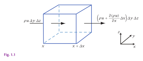
Mass conservation in an rectangular Eulerian control volume. The mass convergence, (plus contributions in the and direct — Figure 4.1.
Mass conservation in an rectangular Eulerian control volume. The mass convergence, $\partial(\rho u)/\partial x$ (plus contributions in the $y$ and $z$ directions), must be balanced by a density decrease. This is Fig. 1.1 in AOFD (Vallis, 2017).

\int_V \frac{\partial \rho}{\partial t} dV = \rho u \Delta y \Delta z - \left(\rho u + \frac{\partial (\rho u)}{\partial x} \Delta x\right) \Delta y \Delta z

\int_V \frac{\partial \rho}{\partial t} dV = - \frac{\partial (\rho u)}{\partial x} \Delta x \Delta y \Delta z

Now, if we allow the flow field to have components in the $y$ and $z$ directions as well, the equation becomes:

\int_V \frac{\partial \rho}{\partial t} dV = - \left[\frac{\partial (\rho u)}{\partial x} + \frac{\partial (\rho v)}{\partial y} + \frac{\partial (\rho w)}{\partial z} \right] \Delta V

Let $\Delta V \to 0$ to such that any field within $\Delta V$ is uniform to obtain:

\frac{\partial \rho}{\partial t} + \nabla \cdot (\rho \mathbf{u}) = 0

This is the continuity equation in the Eulerian reference frame.

We’re not constrained to a rectangular, fixed volume, however. We can derive this equation for an arbitrary control volume using the divergence theorem. The total rate of change of that volume as it moves with the fluid is equal to the surface integral of the velocity field $\mathbf{u}$ through the surface $S$ that is bounding the volume $V$ (Fig. 4.2). Mathematically, we can express this as:

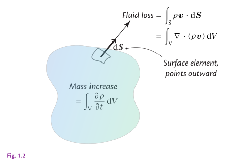
Mass conservation in an arbitrary Eulerian control volume bounded by a surface . The mass increase, is equal to the mass — Figure 4.2.
Mass conservation in an arbitrary Eulerian control volume $V$ bounded by a surface $S$ . The mass increase, $\int_V(\partial \rho/\partial t)dV$ is equal to the mass flowing into the volume, $-\int_S(\rho\mathbf{v}) \cdot d\mathbf{S} = -\int_V \nabla \cdot (\rho\mathbf{v})dV$ . This is Fig. 1.2 in AOFD (Vallis, 2017).

\int_V \frac{\partial \rho}{\partial t} dV = - \int_S \rho \mathbf{u} \cdot d\mathbf{S}

Now, recall the divergence theorem (Eq. 2.28) to obtain:

\int_V \frac{\partial \rho}{\partial t} dV = - \int_V \nabla \cdot (\rho \mathbf{u}) dV

Let $\Delta V \to 0$ to integrate and drop $\Delta V$ on both sides to obtain Eq. 4.4, which is the Eulerian form of the continuity equation.

Lagrangian derivation

In the Lagrangian frame, we follow a fluid parcel as it moves through space. Its mass $\rho \Delta V$ is constant by definition, but its density or volume may change. Since the mass of the parcel is constant, its Lagrangian derivative is zero:

\frac{d}{dt} (\rho \Delta V) = 0

Since the mass doesn’t change, any change in the density of the parcel must be balanced by a change in its volume:

\Delta V \frac{d\rho}{dt} + \rho \frac{d\Delta V}{dt} = 0

Recall that we’ve already derived the Lagrangian derivative of a volume of the fluid parcel (Eq. 3.9), which is the second term here. The equation becomes:

\Delta V \frac{d\rho}{dt} + \Delta V \rho \nabla \cdot \mathbf{u} = 0

Finally, drop $\Delta V$ on both sides to obtain the Lagrangian form of the continuity equation:

\frac{d\rho}{dt} + \rho \nabla \cdot \mathbf{u} = 0

Equations 4.4 and 4.10 are two fundamental expressions of the conservation of mass for a fluid. In one form or another, this equation is a critical component of all weather, ocean, and climate prediction models.

Continuity of an incompressible fluid

Liquids are nearly incompressible, and for them $\frac{d\rho}{dt} = 0$ is a good approximation. For an incompressible fluid, the continuity equation simplifies to:

\nabla \cdot \mathbf{u} = 0

Although as simple as it gets, Eq. 4.11 is extremely important in fluid dynamics.

Conservation of momentum

Like the conservation of mass, the conservation of momentum is a fundamental concept in fluid mechanics. It allows us to predict how the fluid should accelerate due to its state (i.e. velocity and density) and due to the forces acting on it. Together, the continuity and momentum conservation equations form the core of most fluid prediction models, such as weather, ocean, and climate prediction models. We will derive the momentum equation in the remainder of this section. We’ll start from the most basic form first and then incrementally introduce some common forces, such as the pressure gradient force, gravity, and viscosity.

The first step

To derive the momentum conservation equation, we will start from the second Newton’s law, which states that the time rate of change of the momentum of a fluid particle is equal to the net force acting on it. For a fluid parcel of volume $\Delta V = \int_V dV$ whose momentum per unit mass is $\rho \mathbf{u}$ , the momentum conservation equation is:

\frac{d}{dt} \int_V \rho \mathbf{u} dV = \int_V \mathbf{F} dV

where $\mathbf{F}$ is the net force per unit volume acting on the fluid parcel. Let again the volume parcel be very small such that its density and net force acting on it are uniform. We have:

\rho \frac{d\mathbf{u}}{dt} \Delta V = \mathbf{F} \Delta V

\rho \frac{d\mathbf{u}}{dt} = \mathbf{F}

Recall the Lagrangian derivative operator from Eq. 3.5 to obtain:

\frac{\partial \mathbf{u}}{\partial t} + \mathbf{u} \cdot \nabla \mathbf{u} = \frac{\mathbf{F}}{\rho}

This equation states that the acceleration of a fluid parcel at any fixed point in space is equal to the net force per unit mass acting on it, divided by the fluid density. The second term on the left-hand side is the advection term. It represents the local acceleration of the fluid parcel due to the properties of the fluid flow itself. Consider for example a 1-dimensional flow such that the advection term reduces to $u \frac{\partial u}{\partial x}$ . Notice that the advection term is zero only in two special cases: when the velocity is zero or when the velocity is spatially uniform. In all other cases the advection term is non-zero and contributes to the local acceleration.

Because the advection term is velocity multiplied by its gradient, it is nonlinear. This single property of this term makes accurate analysis and prediction of fluid flows difficult. For example, the nonlinear advection term is responsible for the existence of chaos in fluid flows, where small differences in initial conditions lead to vastly different outcomes (in popular culture known as the butterfly effect). One consequence of this in our daily lives is that weather predictability is limited to a finite lead time horizon, for example one to two weeks depending on the weather patterns of interest. If, however, we could assume that either the velocity or its gradient are so small that they could be neglected, the equation simplifies significantly and often allows for analytical solutions. $\mathbf{u} \cdot \nabla \mathbf{u}$ is the most important term for turbulence, weather prediction and predictability, and a major obstacle toward analytical solutions of Eq. 4.15 and its variants. Remember this now.

Back to our equation. For a 3-dimensional Cartesian flow where the velocity field is $\mathbf{u} = (u, v, w)$ and net forces are $\mathbf{F} = (F_x, F_y, F_z)$ , Eq. 4.15 becomes a system of three equations, one for each component of the velocity field. Recall from the Lagrangian derivative operator that $\mathbf{u} \cdot \nabla \mathbf{u}$ is an operator acting on $\mathbf{u}$ (as opposed to divergence of a gradient). The $\mathbf{u} \cdot \nabla$ operator then expands to $u\frac{\partial}{\partial x} + v\frac{\partial}{\partial y} + w\frac{\partial}{\partial z}$ . Our vector equations becomes a system of three scalar equations:

\frac{\partial u}{\partial t} + u \frac{\partial u}{\partial x} + v \frac{\partial u}{\partial y} + w \frac{\partial u}{\partial z} = \frac{F_x}{\rho}

\frac{\partial v}{\partial t} + u \frac{\partial v}{\partial x} + v \frac{\partial v}{\partial y} + w \frac{\partial v}{\partial z} = \frac{F_y}{\rho}

\frac{\partial w}{\partial t} + u \frac{\partial w}{\partial x} + v \frac{\partial w}{\partial y} + w \frac{\partial w}{\partial z} = \frac{F_z}{\rho}

Each of the prognostic equations for the velocity components thus has exactly three advective components that correspond to the gradients of the velocity in each respective direction.

Incorporating the forces

Now we should consider what forces may be acting on the fluid. We distinguish between two types of forces: surface forces and body forces. Surface forces act on the surface of the fluid parcel due to the motion of the fluid molecules, in all directions at that surface. For example, organized motion of molecules into the surface may cause pressure on that surface, and the sheared motion of molecules (e.g. if flow is antiparallel to the surface) may cause shear stress on the surface, leading to the deformation of the fluid parcel. In contrast, body forces act remotely (meaning, from a distance) on the entire volume of the fluid parcel because that parcel is immersed in one or more force fields. Gravity is one such body force, and it’s the only one we’ll consider here. Although in Eq. 4.15 we wrote the net force as $\mathbf{F}$ , it’s useful to write it as the sum of body forces $\mathbf{F}_b$ and surface forces $\mathbf{F}_s$ :

\frac{\partial \mathbf{u}}{\partial t} + \mathbf{u} \cdot \nabla \mathbf{u} = \frac{1}{\rho} (\mathbf{F}_s + \mathbf{F}_b)

Let’s derive the surface forces first. We want to find out the local change of momentum only due to the surface forces. Analogous to how the flow through the volume determined the rate of change of density inside that volume, as we saw in the continuity equation (Eq. 4.4), the change in momentum inside the volume is determined by the surface forces acting on the volume (Fig. 4.3).

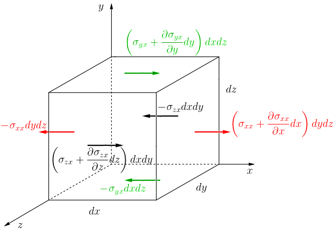
Normal components of the stress tensor acting on a fluid parcel. Reproduced from [https://en.wikipedia.org/wiki/Cauchy_m — Figure 4.3.
Normal components of the stress tensor $\mathbf{\sigma}$ acting on a fluid parcel. Reproduced from https://en.wikipedia.org/wiki/Cauchy_momentum_equation under the CC BY-SA 4.0 license.

Mathematically, we can express this change as:

\int_V \mathbf{F_s} dV = \int_S \boldsymbol{\sigma} \cdot d\mathbf{S}

where $\boldsymbol{\sigma}$ is the second-order stress tensor acting on the surface $S$ of the fluid parcel. As before, recall the divergence theorem (Eq. 2.28) to obtain:

\int_V \mathbf{F_s} dV = \int_V \nabla \cdot \boldsymbol{\sigma} dV

\mathbf{F_s} = \nabla \cdot \boldsymbol{\sigma}

The surface force thus equals the divergence of the stress tensor. Insert this into Eq. 4.15 to get our new form of the momentum equation:

\frac{\partial \mathbf{u}}{\partial t} + \mathbf{u} \cdot \nabla \mathbf{u} = \frac{1}{\rho} \nabla \cdot \boldsymbol{\sigma} + \frac{\mathbf{F}_b}{\rho}

This form of the momentum equation is often called the Cauchy momentum equation.

Let’s now look at what this stress tensor divergence term $\nabla \cdot \boldsymbol{\sigma}$ is.

Pressure gradient

There is a fundamental difference in the meaning of the diagonal and off-diagonal components of the stress tensor. The diagonal components of the stress tensor, $\sigma_{xx}$ , $\sigma_{yy}$ , and $\sigma_{zz}$ , represent the normal stress components, i.e. the force per unit area acting on a surface element that is oriented in the $x$ , $y$ , and $z$ directions, respectively. The off-diagonal components of the stress tensor represent the shear stress components, each acting on all three surfaces. For example, $\sigma_{xy}$ represents the $x$ -component of the stress tensor acting on the surface that is perpendicular to the $y$ -axis. Let’s write out the stress tensor in Cartesian coordinates:

\boldsymbol{\sigma} = \begin{bmatrix} \sigma_{xx} & \sigma_{xy} & \sigma_{xz} \\ \sigma_{yx} & \sigma_{yy} & \sigma_{yz} \\ \sigma_{zx} & \sigma_{zy} & \sigma_{zz} \end{bmatrix}

This tensor can be decomposed into its normal and shear components:

\boldsymbol{\sigma} = -p \mathbf{I} + \boldsymbol{\tau}

where $p$ is the pressure, $\mathbf{I}$ is the identity tensor, and $\boldsymbol{\tau}$ is the deviatoric stress tensor, or, the viscous shear stress tensor. Written out explicitly in Cartesian coordinates and using Eq. 4.25, the stress tensor is:

\boldsymbol{\sigma} = \begin{bmatrix} -p + \tau_{xx} & \tau_{xy} & \tau_{xz} \\ \tau_{yx} & -p + \tau_{yy} & \tau_{yz} \\ \tau_{zx} & \tau_{zy} & -p + \tau_{zz} \end{bmatrix}

The divergence of the stress tensor is then:

\nabla \cdot \boldsymbol{\sigma} = - \nabla p + \nabla \cdot \boldsymbol{\tau}

Let’s insert this into Eq. 4.15 to get our new form of the momentum equation:

\frac{\partial \mathbf{u}}{\partial t} + \mathbf{u} \cdot \nabla \mathbf{u} = - \frac{1}{\rho} \nabla p + \frac{1}{\rho} \nabla \cdot \boldsymbol{\tau} + \frac{\mathbf{F}_b}{\rho}

Pressure is one of the fluid properties that determine its state. Collective, organized, motion of molecules at a macroscopic scale induces pressure on a surface and an associated force acting normal to that surface. Recall that the surface vector is normal to the surface and pointing outward, and the force acting on the fluid surface is oriented inward, thus the minus sign.

In an ideal, inviscid fluid, that is, a fluid that exhibits no viscous forces, the stress tensor $\boldsymbol{\sigma}$ is only composed of the diagonal terms (pressure), and the divergence of the stress tensor is zero. Dropping $\nabla \cdot \boldsymbol{\tau}$ and the body forces $\mathbf{F}_b$ for now, the Cauchy momentum equation simplifies to:

\frac{\partial \mathbf{u}}{\partial t} + \mathbf{u} \cdot \nabla \mathbf{u} = - \frac{1}{\rho} \nabla p

This form of the momentum equation is often called the Euler equation.

Viscous forces

Now, let’s look at the shear stress tensor divergence $\nabla \cdot \boldsymbol{\tau}$ . Written out explicitly as a matrix of all its components, $\boldsymbol{\tau}$ is:

\boldsymbol{\tau} = \begin{bmatrix} \tau_{xx} & \tau_{xy} & \tau_{xz} \\ \tau_{yx} & \tau_{yy} & \tau_{yz} \\ \tau_{zx} & \tau_{zy} & \tau_{zz} \end{bmatrix}

The diagonal components of the deviatoric stress tensor are the normal stresses, while the off-diagonal components are the shear stresses. The normal stresses are non-zero only in compressible fluids ( $\nabla \cdot \mathbf{u} \neq 0$ ), while the shear stresses are zero in non-viscous flows. The divergence of this tensor, written out explicitly as a matrix of all its components, is:

\nabla \cdot \boldsymbol{\tau} = \begin{bmatrix} \frac{\partial \tau_{xx}}{\partial x} + \frac{\partial \tau_{yx}}{\partial y} + \frac{\partial \tau_{zx}}{\partial z} \\ \frac{\partial \tau_{xy}}{\partial x} + \frac{\partial \tau_{yy}}{\partial y} + \frac{\partial \tau_{zy}}{\partial z} \\ \frac{\partial \tau_{xz}}{\partial x} + \frac{\partial \tau_{yz}}{\partial y} + \frac{\partial \tau_{zz}}{\partial z} \end{bmatrix}

Now, write out 4.28 as a system of three scalar equations, one for each component of the velocity field, and insert the shear stress divergence terms to get:

\frac{\partial u}{\partial t} + u \frac{\partial u}{\partial x} + v \frac{\partial u}{\partial y} + w \frac{\partial u}{\partial z} = - \frac{1}{\rho} \frac{\partial p}{\partial x} + \frac{1}{\rho} \left( \frac{\partial \tau_{xx}}{\partial x} + \frac{\partial \tau_{yx}}{\partial y} + \frac{\partial \tau_{zx}}{\partial z} \right) + \frac{F_x}{\rho}

\frac{\partial v}{\partial t} + u \frac{\partial v}{\partial x} + v \frac{\partial v}{\partial y} + w \frac{\partial v}{\partial z} = - \frac{1}{\rho} \frac{\partial p}{\partial y} + \frac{1}{\rho} \left( \frac{\partial \tau_{xy}}{\partial x} + \frac{\partial \tau_{yy}}{\partial y} + \frac{\partial \tau_{zy}}{\partial z} \right) + \frac{F_y}{\rho}

\frac{\partial w}{\partial t} + u \frac{\partial w}{\partial x} + v \frac{\partial w}{\partial y} + w \frac{\partial w}{\partial z} = - \frac{1}{\rho} \frac{\partial p}{\partial z} + \frac{1}{\rho} \left( \frac{\partial \tau_{xz}}{\partial x} + \frac{\partial \tau_{yz}}{\partial y} + \frac{\partial \tau_{zz}}{\partial z} \right) + \frac{F_z}{\rho}

Each of the prognostic equations for the velocity components thus has exactly one pressure gradient and two shear stress gradient terms, all arising from the surface forces.

Experimentally, it was found that the viscous shear stress tensor $\boldsymbol{\tau}$ is proportional to the gradient of the velocity field, i.e. $\boldsymbol{\tau} = \mu \nabla \mathbf{u}$ . This property of the fluid makes it a so-called Newtonian fluid. The proportionality constant $\mu$ is the dynamic viscosity and depends on the fluid properties and temperature. Inserting this into Eq. 4.28, we get:

\frac{\partial \mathbf{u}}{\partial t} + \mathbf{u} \cdot \nabla \mathbf{u} = - \frac{1}{\rho} \nabla p + \frac{1}{\rho} \nabla \cdot (\mu \nabla \mathbf{u}) + \frac{\mathbf{F}_b}{\rho}

We can further simplify this equation by assuming that the viscosity is constant and that the flow is incompressible. This allows us to neglect the viscous stress gradient term, leading to the Navier-Stokes equation.

\frac{\partial \mathbf{u}}{\partial t} + \mathbf{u} \cdot \nabla \mathbf{u} = - \frac{1}{\rho} \nabla p + \nu \nabla^2 \mathbf{u} + \frac{\mathbf{F}_b}{\rho}

where $\nu = \frac{\mu}{\rho}$ is the kinematic viscosity. The operator $\nabla^2 = \left( \frac{\partial^2}{\partial x^2} + \frac{\partial^2}{\partial y^2} + \frac{\partial^2}{\partial z^2} \right)$ is the Laplacian. It is a second-order differential operator that appears in many partial differential equations, including the heat equation, the wave equation, and the Laplace equation. More on these later.

Let’s now look at the body forces to conclude our derivation.

Gravity

As we mentioned earlier, gravity is the only body force we’ll consider here. The force of gravity per unit mass is given by $\mathbf{g} = (0, 0, -g)$ , where $g$ is the gravitational acceleration. Here we assume that the gravitational acceleration is constant and points downward. Insert this into Eq. 4.36, and assuming incompressibility, we get:

\frac{\partial \mathbf{u}}{\partial t} + (\mathbf{u} \cdot \nabla) \mathbf{u} = - \frac{1}{\rho} \nabla p + \mathbf{g} + \nu \nabla^2 \mathbf{u}

Written out explicitly for each of the three spatial dimensions ( $x$ , $y$ , and $z$ ), we get:

\frac{\partial u}{\partial t} + u \frac{\partial u}{\partial x} + v \frac{\partial u}{\partial y} + w \frac{\partial u}{\partial z} = - \frac{1}{\rho} \frac{\partial p}{\partial x} + \nu \left( \frac{\partial^2 u}{\partial x^2} + \frac{\partial^2 u}{\partial y^2} + \frac{\partial^2 u}{\partial z^2} \right)

\frac{\partial v}{\partial t} + u \frac{\partial v}{\partial x} + v \frac{\partial v}{\partial y} + w \frac{\partial v}{\partial z} = - \frac{1}{\rho} \frac{\partial p}{\partial y} + \nu \left( \frac{\partial^2 v}{\partial x^2} + \frac{\partial^2 v}{\partial y^2} + \frac{\partial^2 v}{\partial z^2} \right)

\frac{\partial w}{\partial t} + u \frac{\partial w}{\partial x} + v \frac{\partial w}{\partial y} + w \frac{\partial w}{\partial z} = - \frac{1}{\rho} \frac{\partial p}{\partial z} - g + \nu \left( \frac{\partial^2 w}{\partial x^2} + \frac{\partial^2 w}{\partial y^2} + \frac{\partial^2 w}{\partial z^2} \right)

This completes the full system of momentum conservation equations in the Cartesian coordinate system.

Hydrostatic balance

Take Eq. 4.40 and assume that the vertical acceleration $\frac{dw}{dt}$ is small compared to $g$ , and that the spatial variations of $w$ are small. We can then drop the $\frac{dw}{dt}$ and $\nu \nabla^2 w$ terms to get the hydrostatic approximation:

\frac{\partial p}{\partial z} = - \rho g

which states that the vertical pressure gradient is governed by the density of the fluid and the gravitational acceleration. It’s often a good approximation for large-scale atmospheric and oceanic flows, where the vertical variations of the horizontal velocity components are much smaller than the horizontal variations of the vertical velocity component. Notice however that the hydrostatic approximation does not imply that there is no vertical motion or that it does not vary over time. Instead, according to the continuity equation (Eq. 4.10), it means that the vertical motion is completely governed by the change in density and the divergence of the horizontal velocity field. Further, if the flow is incompressible ( $\nabla \cdot \mathbf{u} = 0$ ), we get:

\frac{\partial w}{\partial z} = - \frac{\partial u}{\partial x} - \frac{\partial v}{\partial y}

which relates the vertical acceleration to the horizontal divergence. Integrating this equation vertically allows us to calculate the vertical velocity anywhere in the fluid column provided bottom and top boundary conditions:

w\left(z\right) = w\left(z+\Delta z\right) - \int_z^{z+\Delta z} \left(\frac{\partial u}{\partial x} + \frac{\partial v}{\partial y} \right) dz'

This relationship will prove to be extremely useful in ocean applications where only the horizontal velocity field is resolved. For example, a group of ocean surface drifters converging towards a region is indicative of downwelling (downward motion in the ocean) in that region. Another example is that of ocean circulation models, which are typically designed as hydrostatic. In the case of such models, the horizontal components of the velocity are prognostic variables, and the vertical velocity is diagnosed using Eq. 4.42.

Equation of state

Now that we have derived the mass and momentum conservation equations, let’s write them out together in vector form:

\frac{\partial \mathbf{u}}{\partial t} + (\mathbf{u} \cdot \nabla) \mathbf{u} = - \frac{1}{\rho} \nabla p + \mathbf{g} + \nu \nabla^2 \mathbf{u}

\frac{\partial \rho}{\partial t} + \nabla \cdot (\rho \mathbf{u}) = 0

Momentum and mass conservation equations are prognostic equations for the vector velocity field $\mathbf{u}$ and the scalar density field $\rho$ , respectively. Notice the one remaining unknown: the scalar pressure field $p$ . As of now, we have a system of two independent equations for the three unknowns: $\mathbf{u}$ , $p$ , and $\rho$ . We need one more equation to close the system—the equation of state—to relate the pressure to the other properties of the fluid, such as temperature, density, and composition.

The prognostic equations that we have derived so far describe equally well the evolution of both the atmosphere and the ocean, despite their significant differences. The equation of state is where our systems of governing equations for the ocean and the atmosphere begin to diverge. Namely, the atmosphere is a mixture of dry air and water vapor, and the ocean is composed of liquid water with varying amounts of dissolved salts. These differences will reflect in the choice of the equation of state to use in each of these systems.

In the atmosphere

In the atmospheres, ideal gas law is often used as the equation of state:

p = \rho R T

where $R$ is the specific gas constant for the gas in question, and $T$ is the temperature. For the moist air, we need to account for both the properties of dry air ( $R_d \approx\ 287\ J kg^{-1} K^{-1}$ ) and those of water vapor ( $R_v \approx\ 461\ J kg^{-1} K^{-1}$ ). The equation of state for moist air relies on the so-called virtual temperature to account for the moisture in the air:

p = \rho R_d T_v

where:

T_v = T \left[1 + q \left(\frac{R_v}{R_d} - 1 \right) \right]

where $q$ is the specific humidity of the air. So, the equation of state for moist air is:

p = \rho R_d T \left[1 + q \left(\frac{R_v}{R_d} - 1 \right) \right]

Recall that we intended to close our system of equations by finding the equation for pressure. Although we did solve for pressure, it seems that we introduced two new unknown variables: the temperature $T$ and the specific humidity $q$ . Each of these variables are governed by their own conservation equations, akin to that for density, but with the addition of source and sink terms that control their production and loss:

\frac{\partial T}{\partial t} + (\mathbf{u} \cdot \nabla) T = \dot{S}_T

\frac{\partial q}{\partial t} + (\mathbf{u} \cdot \nabla) q = \dot{S}_q

where $\dot{S}_T$ and $\dot{S}_q$ are the sources and sinks of temperature and specific humidity, respectively. They are governed by a plethora of thermodynamic processes such as radiation, evaporation, condensation, etc.

Although we won’t delve further into the details behind the sources and sinks of temperature and specific humidity in the atmosphere, we can denote these equations as completing the full system of prognostic equations for the atmosphere: Eqs. 4.44, 4.45, 4.49, 4.50, and 4.51. These equations form the basis of many weather and climate prediction models.

In the ocean

Ideal gas law (Eq. 4.46) doesn’t apply to liquids and the equation of state for seawater is not easily derived. Instead, we assume that the ocean is a single-component fluid, and we use the density field $\rho$ as the equation of state.

\rho = \rho(T, S, p) \\ = \rho_0 \left[ 1 - \beta_T(T-T_0) + \beta_S(S-S_0) + \beta_p(p-p_0) \right]

where $\rho_0$ is the reference density at the reference temperature $T_0$ , salinity $S_0$ , and pressure $p_0$ . The coefficients $\beta_T$ , $\beta_S$ , and $\beta_p$ are the thermal expansion coefficient, the saline contraction coefficient, and the pressure coefficient, respectively. This form of the equation of state is a linear equation of state (as in, the dependence of density on temperature, salinity, and pressure each is linear). Dependence of density on temperature and salinity at two different pressure levels is shown in Fig. 4.4. Higher order equations of state are often used for higher accuracy, however they’re out of scope for this course.

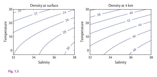
Contours of density as a function of temperature and salinity for seawater. Contour labels are (density - 1000) kg m. Le — Figure 4.4.
Contours of density as a function of temperature and salinity for seawater. Contour labels are (density - 1000) kg m $^{-3}$ . Left panel: at sea-level ( $p = 10^5\ Pa$ , or 1000 mb). Right panel: at $p = 4 \times 10^7\ Pa$ (about 4 km depth). In both cases the contours are slightly convex, so that if two parcels at the same density but different temperatures and salinities are mixed, the resulting parcel is of higher density. (The average temperature is not exactly conserved on mixing, but it very nearly is.) This is Fig. 1.3 in AOFD (Vallis, 2017).

Like we did in the case of atmosphere, here we need to additional prognostic equations, one of temperature and another for salinity:

\frac{\partial T}{\partial t} + (\mathbf{u} \cdot \nabla) T = \dot{S}_T

\frac{\partial S}{\partial t} + (\mathbf{u} \cdot \nabla) S = \dot{S}_S

where $\dot{S}_T$ and $\dot{S}_S$ are the sources and sinks of water temperature and salinity, respectively.

Equations 4.44, 4.45, 4.52, 4.53, and 4.54 are the governing equations used in most numerical ocean circulation models.

Nondimensionalization and scaling

A useful technique to simplify the analysis of the governing equations is to scale the variables using characteristic values for each of the variables. This is known as nondimensionalization or scaling the equations. In practice, for each (dependent or independent) variable $x$ in the equations, we define a characteristic value $X$ . For example, for the velocity $\mathbf{u}$ , we may pick the characteristic value of $U = 1$ m/s or $U = 10$ m/s for the ocean or atmosphere, respectively. We then divide each term in the equations by the characteristic value to obtain a nondimensional (unitless) number. This helps us identify the important parameters that govern the behavior of the system and to group terms in the equations that are of similar magnitudes. This is especially useful for large-scale flows, where the length and time scales can vary over several orders of magnitude.

Let’s look, for example, at the vector equation for horizontal momentum (thus, ignoring $\mathbf{g}$ for now):

\frac{\partial \mathbf{u}}{\partial t} + (\mathbf{u} \cdot \nabla) \mathbf{u} = - \frac{1}{\rho} \nabla p + \nu \nabla^2 \mathbf{u}

The characteristic scales for each term are:

\frac{\partial \mathbf{u}}{\partial t} \sim \frac{U}{T}

(\mathbf{u} \cdot \nabla) \mathbf{u} \sim \frac{U^2}{L}

- \frac{1}{\rho} \nabla p \sim \frac{1}{\rho} \frac{P}{L}

\nu \nabla^2 \mathbf{u} \sim \nu \frac{U}{L^2}

where $U$ , $T$ , $L$ , and $P$ are the characteristic scales for the velocity, time, length, and pressure, respectively. So, if for a given flow we can estimate these characteristic values, we can easily determine which terms are important and which can be neglected. This is the basis of scaling arguments in fluid mechanics.

This approach also enables characterizing the flows in terms of nondimensional numbers. For example, to describe how turbulent or laminar a flow is, it’s useful to relate the inertial to the viscous terms in the momentum equation. Their ratio is called the Reynolds number:

\frac{(\mathbf{u} \cdot \nabla) \mathbf{u}}{\nu \nabla^2 \mathbf{u}} \sim \frac{\frac{U^2}{L}}{\frac{\nu U}{L^2}} = \frac{UL}{\nu} \equiv \text{Re}

You see that the Reynolds number is proportional to the velocity and length scales each, and inversely proportional to the viscosity. A larger Reynolds number corresponds to a more turbulent flow.

Exercises

Derive the Lagrangian form of the continuity equation from the Eulerian form and vice versa. What is the key equation that relates the two forms?
Consider two opposing, horizontal, surface currents along the $x$ -axis. In the vertical they uniformly span a mixed layer that extends from the surface to the depth of 20 meters, with a magnitude of 1 m s $^{-1}$ . The two currents meet at a stagnation zone that is 100 meters wide. Calculate the downwelling velocity at the bottom of the mixed layer. Assume $\nabla \cdot \mathbf{u} = 0$ , no change in mean sea level, and no flow in the $y$ -direction.
Write out the Cauchy, Euler, and Navier-Stokes equations in vector form and discuss their similarities and differences. Give examples of flows that are well described by each of these equations.
Write a computer program that calculates the divergence of a second-order tensor in a Cartesian, 3-dimensional coordinate system.
Write a function in your favorite programming language that takes a value of temperature, salinity, and pressure and returns the density of seawater. Assume linear dependence of density on temperature, salinity, and pressure. Take the thermal expansion coefficient to be $\beta_T = 1.67 \times 10^{-4} K^{-1}$ , the Haline contraction coefficient to be $\beta_S = 7.8 \times 10^{-4} g\ kg^{-1}$ , and the compressibility coefficient to be $\beta_p = 4.4 \times 10^{-10} Pa^{-1}$ . Take the reference density to be $\rho_0 = 1027\ kg\ m^{-3}$ , the reference temperature to be $T_0 = 283\ K$ , the reference salinity to be $S_0 = 35 g\ kg^{-1}$ , and the reference pressure to be $p_0 = 10^5\ Pa$ . When you implement your function, calculate the density of seawater for the range of temperatures from -2 to 30 degrees Celsius, and salinities from 20 to 40 g/kg, and plot it as a contour plot as a function of temperature and salinity. Make such plots for pressure values of $10^5$ , $10^6$ , and $10^7$ Pa.
Calculate the Reynolds number for: (a) a synoptic-scale mid-latitude cyclone in the atmosphere; (b) an mesoscale ocean eddy; (c) a river inflow into the ocean; (d) a breaking ocean surface wave; (e) water flowing through a pipe with a diameter of 0.1 m and flow speed of 1 m s $^{-1}$ . Assume $\nu = 10^{-5} m^2 s^{-1}$ for air and $\nu = 10^{-6} m^2 s^{-1}$ for water.

Summary

In this chapter, we covered:

Conservation of mass (continuity equation) from both Eulerian and Lagrangian perspectives;
Conservation of momentum equations: Cauchy, Euler, and Navier-Stokes;
The Reynolds number as a measure of the relative importance of inertial to viscous forces in a flow;
The equation of state for seawater, relating density to temperature, salinity, and pressure;
Examples of flows with different Reynolds numbers, from laminar pipe flow to turbulent geophysical flows.