Chapter 5

Rotating flows

Fluids behave somewhat differently when in a rotating reference frame, for example on the surface of a rotating planet while being observed from a fixed location on that surface. In this chapter we explore the effects of rotation on the flow. We begin by deriving the temporal derivative of a general vector in a rotating reference frame, and then apply it to find the velocity and acceleration in such a frame. From there we derive the centrifugal and Coriolis forces, and discuss their implications for geophysical flows.

Rate of change of a rotating vector

Before determining what the velocity and acceleration should appear like in a rotating reference frame (i.e. on the surface of a rotating planet), we first need to understand how a vector that is fixed in the rotating frame appears to change over time to the observer in the inertial (fixed) frame. To do that, consider a vector $\mathbf{C}$ that rotates around an axis at a constant angular velocity $\mathbf{\Omega}$ (Fig. 5.1). The angular velocity $\mathbf{\Omega}$ is the rate of change of the angle in the plane that is perpendicular to the axis of rotation, and is thus $\frac{d\lambda}{dt}$ . A unit vector $\mathbf{m}$ is oriented in the direction of the rate of change of $\mathbf{C}$ , and is perpendicular to both $\mathbf{C}$ and $\mathbf{\Omega}$ . We will assume that $\mathbf{\Omega}$ is constant. This is a generally good assumption for the rotation rates of planets, at least on time scales that we are interested in. A small change in $\mathbf{C}$ can then be expressed as:

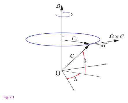
A vector rotating at an angular velocity . It appears to be a constant vector in the rotating frame, whereas in the iner — Figure 5.1.
A vector $\mathbf{C}$ rotating at an angular velocity $\mathbf{\Omega}$ . It appears to be a constant vector in the rotating frame, whereas in the inertial frame it rotates according to $\left(d\mathbf{C}/dt\right)_I = \mathbf{\Omega} \times \mathbf{C}$ . This is Fig. 2.1 in AOFD (Vallis, 2017).

\delta \mathbf{C} = |\mathbf{C}| \cos\theta\ \delta \lambda\ \mathbf{m}

The change in $\mathbf{C}$ is thus proportional to: its magnitude; the cosine of the angle between $\mathbf{C}$ and the horizontal plane (i.e. the plane perpendicular to $\mathbf{\Omega}$ ); the change in $\lambda$ ; and, the unit vector $\mathbf{m}$ . Notice now that using the definition of the cross product (Eq. 2.12), and recalling that $\Omega = \frac{d\lambda}{dt}$ , we can write the change in $\mathbf{C}$ as:

\delta \mathbf{C} = |\mathbf{C}| |\mathbf{\Omega}| \sin(\pi/2 - \theta)\ \mathbf{m}\ \delta t = \mathbf{\Omega} \times \mathbf{C}\ \delta t

so the rate of change of a rotating vector, when observed from a fixed, inertial frame is the cross product of the angular velocity and the vector itself:

\left(\frac{d\mathbf{C}}{dt}\right)_I = \mathbf{\Omega} \times \mathbf{C}

Going forward, we will use the subscript $I$ to denote the inertial frame, non-rotating reference frame.

Imagine now that you’re standing on top of the rotating vector $\mathbf{C}$ , and are still relative to that rotating reference frame, much like standing still on the surface of a rotating planet. To you as the observer in the rotating frame, the vector $\mathbf{C}$ appears to not change in any way. Consider now another vector $\mathbf{B}$ that may change (in direction or magnitude, or both) in the rotating reference frame. We can then say that the rate of change of $\mathbf{B}$ in the inertial frame is the vector sum of its two rates of change: The rate of change of $\mathbf{B}$ in the rotating frame, and the rate of change of the rotating frame itself:

\left(\frac{d\mathbf{B}}{dt}\right)_I = \left(\frac{d\mathbf{B}}{dt}\right)_R + \mathbf{\Omega} \times \mathbf{B}

We now have a useful tool to use to determine the velocity and acceleration in a rotating frame, such as that of of the surface of a rotating planet.

Velocity and acceleration in a rotating frame

Consider now a position vector $\mathbf{r}$ that locates a parcel in the rotating frame. The velocity of the parcel in the inertial frame is then given by the rate of change of the position vector. Apply Eq. 5.4 to $\mathbf{r}$ to get:

\left( \frac{d\mathbf{r}}{dt} \right)_I = \left( \frac{d\mathbf{r}}{dt} \right)_R + \mathbf{\Omega} \times \mathbf{r}

As the time derivative of a position vector is velocity by definition, we can write this as:

\mathbf{u}_I = \mathbf{u}_R + \mathbf{\Omega} \times \mathbf{r}

This relates the inertial and rotating velocities. Recall that we are interested in accelerations, as it’s the acceleration that we solve for in the Navier-Stokes equations and relate to the forces that act on the fluid. We know that the acceleration is the rate of change of velocity, so let’s apply Eq. 5.4 to the rotating velocity:

\left( \frac{d\mathbf{u}_R}{dt} \right)_I = \left( \frac{d\mathbf{u}_R}{dt} \right)_R + \mathbf{\Omega} \times \mathbf{u}_R

Now, use Eq. 5.6 to substitute for $\mathbf{u}_I$ in Eq. 5.7:

\left( \frac{d\left(\mathbf{u}_I - \mathbf{\Omega} \times \mathbf{r}\right)}{dt} \right)_I = \left( \frac{d\mathbf{u}_R}{dt} \right)_R + \mathbf{\Omega} \times \mathbf{u}_R

\left( \frac{d \mathbf{u}_I}{dt} \right)_I = \left( \frac{d \mathbf{u}_R}{dt} \right)_R + \mathbf{\Omega} \times \mathbf{u}_R + \frac{d\mathbf{\Omega}}{dt} \times \mathbf{r} + \mathbf{\Omega} \times \left( \frac{d\mathbf{r}}{dt} \right)_I

Recall that:

\left( \frac{d \mathbf{r}}{dt} \right)_I = \left( \frac{d \mathbf{r}}{dt} \right)_R + \mathbf{\Omega} \times \mathbf{r} = \mathbf{u}_R + \mathbf{\Omega} \times \mathbf{r}

If $\mathbf{\Omega}$ is constant, as we have assumed at the beginning, inserting Eq. 5.10 into Eq. 5.9 yields:

\left( \frac{d \mathbf{u}_R}{dt} \right)_R = \left( \frac{d \mathbf{u}_I}{dt} \right)_I - 2 \mathbf{\Omega} \times \mathbf{u}_R - \mathbf{\Omega} \times \left( \mathbf{\Omega} \times \mathbf{r} \right)

The interpretation of the terms in Eq. 5.11 is:

$\left( \frac{d \mathbf{u}_R}{dt} \right)_R$ , is the rate of change of the relative velocity as observed in the rotating frame. This is the rate of change of the velocity that you would measure with an anemometer or current meter if position fixed relative to the rotating planet’s surface.
$\left( \frac{d \mathbf{u}_I}{dt} \right)_I$ , is the rate of change of the inertial velocity, i.e. the velocity as observed in the inertial frame.
$-2 \mathbf{\Omega} \times \mathbf{u}_R$ , is the Coriolis acceleration . The Coriolis acceleration (and correspondingly, the Coriolis force) is responsible for the organized rotation of large-scale atmospheric and oceanic flows. Notice that the Coriolis acceleration is always perpendicular to the relative velocity $\mathbf{u}_R$ . This means that whenever we have a flow in a rotating frame, the Coriolis force deflects the flow to the right or the left depending on the orientation of $\Omega$ relative to the plane of the flow (i.e. the deflection is to the right on the northern hemisphere and to the left on the southern hemisphere).
$-\mathbf{\Omega} \times \left( \mathbf{\Omega} \times \mathbf{r} \right)$ , is the centrifugal acceleration. It’s always antiparallel to the position vector $\mathbf{r}$ by definition. Notice also that the centrifugal acceleration is not dependent on the velocity of the parcel, but only on its position and the angular velocity of the rotating frame. This force could then be considered a body force, much like gravity. Indeed, for practical reasons, centrifugal force if often bundled together with gravitational force and expressed as a gradient of the scalar potential $\Phi$ :

$\mathbf{g} - \mathbf{\Omega} \times \mathbf{\Omega} \times \mathbf{r} \equiv - \nabla \Phi$
Effects of the centrifugal force on the effective gravity is illustrated in Fig. 5.2.

If we bundle the centrifugal and the gravitational accelerations together and express them as a geopotential gradient, we can write our momentum balance with the effects of rotation as:

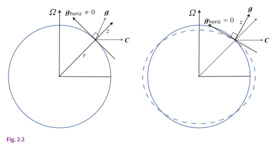
\frac{\partial \mathbf{u}}{\partial t} + \left( \mathbf{u} \cdot \nabla \right) \mathbf{u} = - \frac{1}{\rho} \nabla p - \nabla \Phi - 2 \mathbf{\Omega} \times \mathbf{u} + \nu \nabla^2 \mathbf{u}

Left: directions of forces and coordinates in true spherical geometry. is the effective gravity (including the centrifug — Figure 5.2.
Left: directions of forces and coordinates in true spherical geometry. $\mathbf{g}$ is the effective gravity (including the centrifugal force, $\mathbf{C}$ ) and its horizontal component is evidently non-zero. Right: a modified coordinate system, in which the vertical direction is defined by the direction of $\mathbf{g}$ , and so the horizontal component of $\mathbf{g}$ is identically zero. The dashed line schematically indicates a surface of constant geopotential. The differences between the direction of $\mathbf{g}$ and the direction of the radial coordinate, and between the sphere and the geopotential surface, are much exaggerated and in reality are similar to the thickness of the lines themselves. This is Fig. 2.2 in AOFD (Vallis, 2017).

Coriolis force components

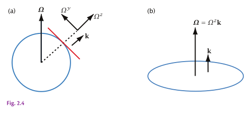
(a) On the sphere the rotation vector can be decomposed into two components, one in the local vertical and one in the lo — Figure 5.3.
(a) On the sphere the rotation vector $\mathbf{\Omega}$ can be decomposed into two components, one in the local vertical and one in the local horizontal, pointing toward the pole. That is, $\mathbf{\Omega} = \Omega_y \mathbf{j} + \Omega_z \mathbf{k}$ where $\Omega_y = \Omega \cos\theta$ and $\Omega_z = \Omega \sin\theta$ . In geophysical fluid dynamics, the rotation vector in the local vertical is often the more important component in the horizontal momentum equations. On a rotating disk, (b), the rotation vector $\mathbf{\Omega}$ is parallel to the local vertical $\mathbf{k}$ . This is Fig. 2.4 in AOFD (Vallis, 2017).

Let’s now examine in more detail the effects the Coriolis force on the flow. The angular velocity $\mathbf{\Omega}$ is a vector that points in the direction oriented from the center of the Earth toward the North Pole (see Fig. 5.3). On the surface of the planet, thus, it has two components: A locally vertical one, $\Omega_z$ , and a meridional one, $\Omega_y$ :

\mathbf{\Omega} = \begin{bmatrix} 0 \\ \Omega_y \\ \Omega_z \end{bmatrix} = \begin{bmatrix} 0 \\ \Omega \cos\theta \\ \Omega \sin\theta \end{bmatrix}

where $\theta$ is the latitude.

The Coriolis force is then:

- 2 \mathbf{\Omega} \times \mathbf{u} = \begin{bmatrix} \mathbf{i} & \mathbf{j} & \mathbf{k} \\ 0 & - 2 \Omega \cos\theta & - 2 \Omega \sin\theta \\ u & v & w \end{bmatrix} = \begin{bmatrix} - 2 \Omega w \cos\theta + 2 \Omega v \sin\theta \\ - 2 \Omega u \sin\theta \\ 2 \Omega u \cos\theta \end{bmatrix}

The Coriolis term thus contributes to all three components of the flow, and their components vary with latitude. Let’s look at the horizontal components first. On geophysical scales, generally $w \ll u$ and so $2 \Omega w \cos\theta$ can often be neglected. The two dominant horizontal components of the Coriolis force then become $(-2\Omega v \sin\theta, 2\Omega u \sin\theta)$ . These components are zero at the Equator and increase poleward. The vertical component, $-2 \Omega u \cos\theta$ , is negligible as well compared to the other terms in the momentum equation, most notably the gravitational acceleration $\mathbf{g}$ and the vertical pressure gradient that balances it. The horizontal effect is thus significantly more relevant for the horizontal motion than the vertical one.

The practical implications of the Coriolis force on the flow is that it deflects it toward the right on the Northern hemisphere and toward the left on the Southern hemisphere. If a parcel or a particle with some initial velocity on a rotating planet is let undisturbed by other forces, it will appear to the observer standing on the surface of the planet to move in circles with some radius. We will calculate soon exactly how big this radius is depending on where on the planet we are and the initial velocity of the parcel. Let’s now incorporate the Coriolis force components into the vector-component form of the momentum equation and apply some convenient approximations, namely the $f$ -plane and the $\beta$ -plane approximations.

$f$ -plane and $\beta$ -plane approximations

Although geophysical fluids flow in a thin layer on a sphere, the curvature of the surface of the planet is negligible for many applications. Here we will make the so-called $f$ -plane approximation in which the flow is assumed to be on a flat plane tangent to the surface of a curved planet. The main assumption of the $f$ -plane approximation is that the planet’s rotation exhibits only a locally vertical component anywhere on that planet’s surface. In other words, we’ll neglect the horizontal component (i.e. $\Omega_y$ ). With that assumption, the Coriolis force becomes strictly horizontal:

- 2 \mathbf{\Omega} \times \mathbf{u} = \begin{bmatrix} 2 \Omega v \sin\theta \\ - 2 \Omega u \sin\theta \\ 0 \end{bmatrix}

Let’s now define the so-called Coriolis parameter $f_0 = 2 \Omega_z = 2 \Omega \sin\theta$ , so we can write the Coriolis force more concisely as:

- f_0 \mathbf{k} \times \mathbf{u} = \begin{bmatrix} f_0 v \\ - f_0 u \\ 0 \end{bmatrix}

The effect of the Coriolis force on the flow is now even more apparent: A positive meridional flow causes a positive zonal acceleration, and a positive zonal flow causes a negative meridional acceleration. The implication of this is that the Coriolis force induces clockwise and counterclockwise rotations in the Northern and Southern hemispheres, respectively.

Ignoring viscosity for brevity, we can re-write our system of momentum equations as:

\frac{du}{dt} = - \frac{1}{\rho} \frac{\partial p}{\partial x} + f_0 v

\frac{dv}{dt} = - \frac{1}{\rho} \frac{\partial p}{\partial y} - f_0 u

\frac{dw}{dt} = - \frac{1}{\rho} \frac{\partial p}{\partial z} - g

While on the small plane tangential to the planet’s surface the local rotation may be uniform in space, in reality it does vary with latitude:

f = 2 \Omega \sin\theta \approx 2\Omega \sin\theta_0 + 2\Omega (\theta - \theta_0) \cos\theta_0

for small deviations in $\theta$ . We obtained this expression by expanding $f$ in a Taylor series to the first order around $\theta_0$ . On a plane, the above can be expressed as:

f = f_0 + \beta y

where $f_0 = 2\Omega \sin\theta_0$ and $\beta = \partial f/\partial y = (2\Omega\cos\theta_0) / R_E$ (where $R_E$ is the radius of the Earth).

Geostrophic balance

Now that we have incorporated the effects of rotation into our equations of motion, let’s evaluate the scales of the terms in the horizontal momentum equations. We will start from Eq. 5.13, use the f-plane notation for the Coriolis term, ignore the viscous terms, and drop the gravity term as we’re looking at the flow in the horizontal plane:

\frac{\partial \mathbf{u}}{\partial t} + (\mathbf{u} \cdot \nabla) \mathbf{u} + \mathbf{f} \times \mathbf{u} = - \frac{1}{\rho} \nabla p

As we did in Section Nondimensionalization and scaling, let’s scale each term on the left-hand side with their characteristic scales for mesoscale ocean flow ( $L \sim 10^5\ m$ , $T \sim 10^6\ s$ , $U \sim 10^{-1}\ m/s$ ):

$\frac{\partial \mathbf{u}}{\partial t} \sim \frac{U}{T} \sim 10^{-7}$
$(\mathbf{u} \cdot \nabla) \mathbf{u} \sim \frac{U^2}{L} \sim 10^{-7}$
$\mathbf{f} \times \mathbf{u} \sim f_0 U \sim 10^{-6}$

This means that on these oceanic scales ( $L \sim 100\ km$ , $T \sim 1\ day$ ), the inertial terms are of the same order of magnitude as the Coriolis term. In other words, rotation here is much more important than the local rate of change or advection. Also, whatever the scale of the pressure gradient term is, it is the only term that can balance the rotation. Thus, if we can state that the inertial terms can be neglected, we can also state:

\mathbf{f} \times \mathbf{u} \approx - \frac{1}{\rho} \nabla p

or, in scalar component form:

f u \approx - \frac{1}{\rho} \frac{\partial p}{\partial y}

f v \approx \frac{1}{\rho} \frac{\partial p}{\partial x}

This balance is called the geostrophic balance, and it is a key concept in geophysical fluid dynamics. It states that the flow is governed by the balance between the rotation and the pressure gradient force. Although the geostrophic balance is strictly an approximation and it never holds exactly, large scale oceanic ( $L \sim 100\ km$ and larger) and atmospheric ( $L \sim 1000\ km$ and larger) flows are often in geostrophic balance. For the analysis of geophysical flows at such scales, it is then useful to define the geostrophic velocity as:

u_g = - \frac{1}{\rho f} \frac{\partial p}{\partial y}

v_g = \frac{1}{\rho f} \frac{\partial p}{\partial x}

Notice that the geostrophic flow is always perpendicular to the pressure gradient, which means it is parallel to the isobars (lines of constant pressure). This also means that the isobars are streamlines of the geostrophic flow. In the northern hemisphere ( $f > 0$ ), the geostrophic flow is cyclonic (counter-clockwise) around the low-pressure region and anti-cyclonic (clockwise) around the high-pressure region. In the southern hemisphere ( $f < 0$ ), it is the opposite. A nearly geostrophic flow is illustrated in Fig. 5.4.

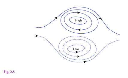
Geostrophic flow with a positive value of the Coriolis parameter . Flow is parallel to the lines of constant pressure (i — Figure 5.4.
Geostrophic flow with a positive value of the Coriolis parameter $f$ . Flow is parallel to the lines of constant pressure (isobars). Cyclonic flow is anticlockwise around a low pressure region and anticyclonic flow is clockwise around a high. If $f$ were negative, as in the Southern Hemisphere, (anti)cyclonic flow would be (anti)clockwise. This is Fig. 2.5 in AOFD (Vallis, 2017).

Rossby number

Recall that we required the inertial terms to be much smaller than the Coriolis term for the geostrophic approximation to hold. Like we did earlier with the Reynolds number to quantify how turbulent a flow is, we can define the Rossby number as:

\text{Ro} \equiv \frac{\text{Advection}}{\text{Rotation}} = \frac{\left( \mathbf{u} \cdot \nabla \right) \mathbf{u}}{\mathbf{f} \times \mathbf{u}} \approx \frac{\frac{U^2}{L}}{fU} \approx \frac{U}{fL}

Although the Rossby number characterizes the relative importance of rotation in the flow, notice that the rotation term is in the denominator. The Rossby number is thus small for flows in which rotation dominates over advection. In general, flows with a Rossby number of 0.1 or smaller are considered approximately geostrophically balanced.

Inertial oscillations

An analytical solution to the linearized horizontal momentum equations with rotation gives rise to a steady circular motion called the inertial oscillation. Start from the linearized horizontal momentum equations with rotation and with the pressure gradient force neglected:

\frac{\partial \mathbf{u}}{\partial t} + \mathbf{f} \times \mathbf{u} = 0

In scalar component form, this is:

\frac{\partial u}{\partial t} + f v = 0

\frac{\partial v}{\partial t} - f u = 0

We are now looking for a solution for ( $u(t), v(t)$ ). These two equations are linear but coupled, so we need to decouple them first to obtain the equations with one unknown variable each. Differentiate each equation with respect to time to get:

\frac{\partial^2 u}{\partial t^2} + f \frac{\partial v}{\partial t} = 0

\frac{\partial^2 v}{\partial t^2} - f \frac{\partial u}{\partial t} = 0

and then insert Eqs. (5.31)-(5.32) into the above to get:

\frac{\partial^2 u}{\partial t^2} + f^2 u = 0

\frac{\partial^2 v}{\partial t^2} + f^2 v = 0

The equations are now decoupled and each is a second-order, linear, homogeneous, ordinary differential equation with constant coefficients. The general solution to these equations is:

u = A \cos(f t) + B \sin(f t)

v = C \cos(f t) + D \sin(f t)

To find the constants $A$ , $B$ , $C$ , and $D$ , take the initial conditions for the velocity to be $\mathbf{u}(t=0) = [u_0, v_0]$ . This results in:

u = u_0 \cos(f t) + v_0 \sin(f t)

v = v_0 \cos(f t) - u_0 \sin(f t)

These equations describe a circular motion in the horizontal plane with a radius of $r_0 = \sqrt{u_0^2 + v_0^2} / f$ and a period of $2\pi / f$ . It can be demonstrated that the motion is circular by integrating the velocities (Eqs. 5.39-5.40) over time to obtain displacements $x(t)$ and $y(t)$ and showing that the displacement radius $r = \sqrt{x^2 + y^2}$ is constant, which can only be true for a circular motion. As the inertial oscillations scale with $1/f$ , they are larger and slower near the Equator and smaller and faster near the poles. For example, at 45 degrees latitude, $f \approx 10^{-4}\ s^{-1}$ , and so the period of the inertial oscillation is $2\pi/f \approx 17.5$ hours.

Exercises

Calculate the effective gravity at the Earth’s Equator, poles, and 45 degrees latitude, taking into effect centrifugal acceleration.
Using scale analysis, show that on geophysical scales the vertical component of the Coriolis force is negligible compared to the other terms in the momentum equation.
Show that the kinetic energy of an inertial oscillation is constant.

Summary

In this chapter, we covered:

The effects of rotation on fluid motion, including centrifugal and Coriolis forces;
Derivation of velocity and acceleration in a rotating reference frame;
The Coriolis parameter $f$ and its variation with latitude;
Inertial oscillations - circular motions that arise from the balance between inertia and Coriolis force;
The solution for inertial oscillations showing circular motion with period $2\pi/f$ and radius $r_0 = \sqrt{u_0^2 + v_0^2}/f$ .