Chapter 6

Stratified flows

Oceans and atmospheres are vertically stratified due to the effects of gravity. In the previous chapters, we derived our equations for mass and momentum conservation and we incorporated the effects of rotation. We also explored how the density may vary in the vertical according to the ideas gas law (in the atmosphere) or the equation of state for seawater. We now explore the effects of density stratification on the flow and examine a common approximation used for large-scale oceanic flows.

The Boussinesq equations

We will now explore within our framework the density perturbations that will allow for buoyancy effects in a flow. The Boussinesq approximation is an approximation to the full equations of motion. It assumes that the density and pressure perturbations are much smaller than their means, and when applied to the Navier-Stokes equations, results in the Boussinesq equations.

To start, we will allow the density to have small variations around its mean value. Decompose the density into the mean and the perturbation components:

\rho = \rho_0 + \delta \rho(x, y, z, t)

where $\rho_0$ is the mean density and $\delta \rho$ is its perturbation. Further, we decompose the pressure as:

p = p_0(z) + \delta p(x, y, z, t)

where $p_0$ is the horizontally and temporally averaged pressure and $\delta p$ is its perturbation. Unlike in the density decomposition, the mean pressure component is allowed to vary in $z$ . For both quantities, we require that their perturbations are much smaller than their respective means, i.e. $\delta \rho \ll \rho_0$ , $\delta p \ll p_0$ . In other words, the pressure vary much more in the vertical than in the horizontal or over time, and any perturbations in density, including those in the vertical, are much smaller than the mean density. This approximation can be demonstrated to hold well by using the equation of state for seawater (Eq. 4.52), for example. The hydrostatic approximation in this framework is trivially satisfied:

\frac{d p_0}{d z} = - \rho_0 g

Now that we’ve established the approximation we need, let’s proceed to apply it to our momentum and continuity equations.

Momentum balance

Let’s first apply the Boussinesq approximation to the momentum balance. Recall the Navier-Stokes equation with rotation (Eq. 5.13), while neglecting the viscosity term:

\frac{d \mathbf{u}}{dt} = - \frac{1}{\rho} \nabla p - f \mathbf{k} \times \mathbf{u} + \mathbf{g}

Apply Eqs. 6.1-6.2 to the above equation to get:

\left( \rho_0 + \delta \rho \right) \left( \frac{d \mathbf{u}}{dt} + \mathbf{f} \times \mathbf{u} \right) = - \nabla \left( p_0 + \delta p \right) + \left( \rho_0 + \delta \rho \right) \mathbf{g}

- \nabla \left( p_0 + \delta p \right) = - \nabla \delta p - \frac{\partial p_0}{\partial z} \mathbf{k} = - \nabla \delta p - \rho_0 \mathbf{g}

Now, recall that $\delta \rho \ll \rho_0$ , so we can drop the $\delta \rho$ on the left-hand side:

\rho_0 \left( \frac{d \mathbf{u}}{dt} + \mathbf{f} \times \mathbf{u} \right) = - \nabla \delta p + \delta \rho\ \mathbf{g}

\frac{d \mathbf{u}}{dt} + \mathbf{f} \times \mathbf{u} = - \frac{1}{\rho_0} \nabla \delta p + \frac{\delta \rho}{\rho_0} \mathbf{g}

For convenience of notation, let’s now define buoyancy as $b = - g \delta \rho / \rho_0$ , and re-write the above to obtain the Boussinesq momentum equation:

\frac{d \mathbf{u}}{dt} + \mathbf{f} \times \mathbf{u} = - \frac{1}{\rho_0} \nabla \delta p + b \mathbf{k}

This equation states that now that we are in a gradually stratified fluid, the gravity term is scaled by $\delta \rho / \rho_0$ to yield the appropriate vertical acceleration, and the pressure gradient is due to the relatively small perturbations in density $\delta \rho$ around the mean density $\rho_0$ .

Continuity

As we did for the momentum equation, we’ll now apply the Boussinesq approximation (i.e. $\rho = \rho_0 + \delta \rho$ , $\delta \rho \ll \rho_0$ ) to the continuity equation. Recall the continuity equation in its complete form:

\frac{d \rho}{dt} + \rho \nabla \cdot \mathbf{u} = 0

Insert Eq. 6.1 to get:

\frac{d\delta \rho}{dt} + \left( \rho_0 + \delta \rho \right) \nabla \cdot \mathbf{u} = 0

Then, if we can state that that $d\delta \rho / dt \ll \rho_0 \nabla \cdot \mathbf{u}$ , which we will for the Boussinesq approximation, we recover the original continuity equation for incompressible flows:

\nabla \cdot \mathbf{u} = 0

Note that we do not say that strictly $d \delta \rho / dt = 0$ , but rather that we can neglect it in this equation in favor of the velocity divergence term. The evolution of $\delta \rho$ is still governed by the evolution of buoyancy, which in turn is governed by the evolution of the temperature and salinity fields and the equation of state. The buoyancy $b = - g \delta \rho / \rho_0$ evolves as:

\frac{d b}{dt} = \dot{b}

and the equation of state can be expressed in terms of buoyancy:

b = b(T, S, p)

which is just another form of Eq. 4.52.

Finally the temperature and salinity evolve as before, following Eqs. 4.53 and 4.54, respectively.

Complete system of equations

The full system of Boussinesq equations for the ocean are then:

\frac{d \mathbf{u}}{dt} + \mathbf{f} \times \mathbf{u} = - \frac{1}{\rho_0} \nabla \delta p + b \mathbf{k}

\nabla \cdot \mathbf{u} = 0

\frac{d T}{dt} = \dot{T}

\frac{d S}{dt} = \dot{S}

b = b(T, S, p)

Thermal wind balance

Now that we regard the ocean as a stratified and rotating fluid with a buoyancy defined as $b = - g \delta \rho / \rho_0$ , an emerging property of the flow appears if we combine this fact with the geostrophic balance (see Section Geostrophic balance). Recall the components of geostrophic velocity (Eqs. 6.20-6.21):

u_g = - \frac{1}{\rho f} \frac{\partial p}{\partial y}

v_g = \frac{1}{\rho f} \frac{\partial p}{\partial x}

Differentiate each with respect to $z$ to get:

\frac{\partial u_g}{\partial z} = - \frac{1}{\rho f} \frac{\partial^2 p}{\partial z \partial y} = - \frac{1}{\rho f} \frac{\partial}{\partial y} \left( \frac{\partial p_0}{\partial z} + \frac{\partial \delta p}{\partial z} \right)

\frac{\partial v_g}{\partial z} = \frac{1}{\rho f} \frac{\partial^2 p}{\partial z \partial x} = \frac{1}{\rho f} \frac{\partial}{\partial x} \left( \frac{\partial p_0}{\partial z} + \frac{\partial \delta p}{\partial z} \right)

Applying the hydrostatic approximation (Eq. 6.3) to the above equations, and recalling the definition of buoyancy, we get:

\frac{\partial u_g}{\partial z} = - \frac{1}{f} \frac{\partial b}{\partial y}

\frac{\partial v_g}{\partial z} = \frac{1}{f} \frac{\partial b}{\partial x}

Equations 6.24-6.25 are known as the thermal wind balance (despite the name, it applies to oceans and atmopsheres alike!). It states that the geostrophic velocity must be vertically sheared in the presence of a horizontal buoyancy (density) gradient. This is illustrated in Fig. 6.1. Warm and light air means $\delta \rho < 0$ and thus $b > 0$ , while cold and dense air means $\delta \rho > 0$ and thus $b < 0$ . By hydrostasy, the vertical gradient of the pressure anomaly $\partial \delta p / \partial z$ is positive on the left and negative on the right. This establishes negative horizontal pressure gradient aloft and a positive one near the ground. As the Coriolis force balances the horizontal pressure gradients, the geostrophic wind is positive aloft (out of the page) and negative near the ground (into the page). Thus, in a geostrophic balanced flow alone, introducing a horizontal buoyancy gradient results in a vertical shear of the horizontal velocity.

Figure 6.1.
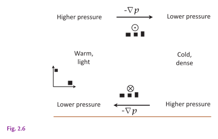
The mechanism of thermal wind. A cold fluid is denser than a warm fluid, so by hydrostasy the vertical pressure gradient is greater where the fluid is cold. Thus, pressure gradients form as shown, where “higher” and “lower” mean relative to the average at that height. The horizontal pressure gradients are balanced by the Coriolis force, producing (for $f > 0$ ) the horizontal winds shown. Only the wind shear is given by the thermal wind. This is Fig. 2.6 in AOFD (Vallis, 2017).

Static instability

We now consider how a fluid parcel may oscillate when its density is perturbed from its resting state and in absence of horizontal flow. This allows us to study the vertical motions due to the vertical differences in density and in isolation from other processes. We will approach this problem by displacing a fluid parcel adiabatically (i.e. without exchange of heat or mass with the environment) by a small distance $\delta z$ and examining how the pressure and gravity forces act on it in response (Fig. 6.2). Recall that in Eq. 6.1 we allowed for the density variations to be much smaller than the mean density, i.e. $\delta \rho \ll \rho_0$ . Here we expand the density decomposition to a finer detail, specifically:

\rho = \rho_0 + \widetilde{\rho}(z) + \delta \rho(x, y, z, t)

where we now differentiate between the mean density $\rho_0$ and the vertically-varying environmental density $\widetilde{\rho}(z)$ , while the perturbation $\delta \rho$ includes the vertical, horizontal, and temporal density variations.

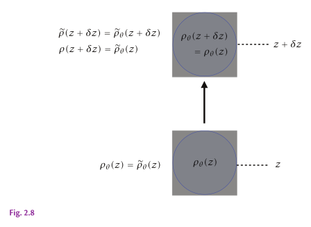
A parcel is adiabatically displaced upward from level to . A tilde denotes the value in the environment, and variables w — Figure 6.2.
A parcel is adiabatically displaced upward from level $z$ to $z + \delta z$ . A tilde denotes the value in the environment, and variables without tildes are those in the parcel. The parcel preserves its potential density, $\rho_\theta$ , which it takes from the environment at level $z$ . If $z + \delta z$ is the reference level, the potential density there is equal to the actual density. The parcel’s stability is determined by the difference between its density and the environmental density. If the difference is positive, the displacement is stable, and if negative the displacement is unstable. This is Fig. 2.8 in AOFD (Vallis, 2017).

As the fluid parcel is displaced adiabatically, its pressure changes instantaneously to assume the same pressure as the environment. However, its temperature and salinity do not change instantaneously, resulting in a density change. To account for the instantaneous change in pressure as the parcel is displaced in height, rather than the actual density we need to consider the parcel’s potential density, $\rho_\theta$ . The potential density is the density the parcel would have if it were returned to the level where the initial pressure was $p_0$ :

\rho_\theta = \rho + \frac{p_0}{c_s^2} = \rho + \frac{\rho_0 g z}{c_s^2}

where $c_s^2 = \left| \partial p / \partial \rho \right|_\theta$ is the square of the speed of sound in the fluid, which we here assume to be constant and equal to $\approx 1500 \, \text{m/s}$ . $c_s^2$ is also related to the pressure compressibility of the fluid in the equation of state for seawater (Eq. 4.52), $\beta_p = 1/(\rho_0 c_s^2)$ . Thus, if the parcel ascends or descends adiabatically, without a change in temperature or salinity, but allowing it to assume environmental pressure, its density will change but its potential density will remain constant. Potential density is thus a useful concept for understanding the static stability of the fluid.

Our goal now is to express a small change in density of the parcel relative to the environment solely in terms of the vertical gradient of the potential density. From Fig. 6.2, we start from:

\delta \rho = \rho(z + \delta z) - \widetilde{\rho}(z + \delta z)

which is the difference between the parcel’s density and the environmental density at the new level. Taking the reference level to be $z + \delta z$ means that:

\rho(z + \delta z) = \rho_\theta(z + \delta z)

so we can re-write the above as:

\delta \rho = \rho_\theta(z + \delta z) - \widetilde{\rho}_\theta(z + \delta z)

Since the parcel’s potential density is conserved during the adiabatic displacement, $\rho_\theta(z) = \rho_\theta(z+\delta z)$ , and recall that at the starting level the parcel’s potential density equals the environmental potential density, i.e. $\rho_\theta(z) = \widetilde{\rho}_\theta(z)$ , we can write:

\delta \rho = \widetilde{\rho}_\theta(z) - \widetilde{\rho}_\theta(z + \delta z)

Then, for small $\delta z$ :

\delta \rho = - \frac{\partial \widetilde{\rho}_\theta}{\partial z} \delta z

The parcel’s static stability is thus determined by the vertical gradient of the locally-referenced potential density of the environment, $\widetilde{\rho_\theta}$ :

\frac{\partial \widetilde{\rho}_\theta}{\partial z} < 0 \quad \text{(statically stable)}

\frac{\partial \widetilde{\rho}_\theta}{\partial z} > 0 \quad \text{(statically unstable)}

Now, to determine the oscillatory motion of the parcel, we apply Newton’s second law and balance the acceleration of the parcel with the buoyancy force:

\frac{\partial^2 \delta z}{\partial t^2} = \frac{g}{\rho} \left( \frac{\partial \widetilde{\rho}_\theta}{\partial z} \right) \delta z = - N^2 \delta z

where we have defined the Brunt-Väisälä frequency (or buoyancy frequency) as:

N^2 = - \frac{g}{\widetilde{\rho}_\theta} \frac{\partial \widetilde{\rho}_\theta}{\partial z} = \frac{d\widetilde{b}}{dz}

while noting that $\rho(z) = \widetilde{\rho}_\theta(z)$ within $\mathcal{O}(\delta z)$ . A parcel displaced from its equilibrium position will oscillate with angular frequency $N$ if $N^2 > 0$ (statically stable), and freely accelerate upward if $N^2 < 0$ (statically unstable). To demonstrate this, we recognize that, like the inertial oscillation equations in Section Inertial oscillations, this is a second-order, linear, homogeneous, ordinary differential equation with constant coefficients. Its general solution is:

\delta z = A \cos(N t) + B \sin(N t), \quad \text{if } N^2 > 0

\delta z = C e^{|N| t} + D e^{-|N| t}, \quad \text{if } N^2 < 0

As before, the values of coefficients $A$ , $B$ , $C$ , and $D$ can be found by applying the initial conditions for $\delta z$ and $d \delta z / dt$ at $t = 0$ . They are $A = \delta z_{t=0}$ , $B = 0$ , $C = D = \delta z_{t=0} / 2$ , assuming that the initial vertical velocity is zero.

\delta z = \delta z_{t=0} \cos(N t), \quad \text{if } N^2 > 0

\delta z = \frac{1}{2} \delta z_{t=0} \left( e^{|N| t} + D e^{-|N| t} \right) = \delta z_{t=0} \cosh(|N| t), \quad \text{if } N^2 < 0

In Python, the solution for the static instability oscillation can be coded like this:

import numpy as np

def parcel_displacement(z0: float, N2: float, t: float) -> float:
    """Given initial parcel displacement z0, buoyancy frequency squared N2,
    return the parcel displacement at time t."""
    N = np.sqrt(complex(N2))
    if N2 > 0:  # stable
        return z0 * np.cos(N * t)
    else:  # unstable
        return z0 * np.cosh(np.abs(N) * t)

This oscillation is illustrated in Fig. 6.3. In stable stratification (top panel), the parcel oscillates around its equilibrium position with frequency $N$ . Higher stratification (larger $N$ ), leads to faster oscillations, while the amplitude is controlled by the initial displacement $\delta z_{t=0}$ . In unstable stratification (bottom panel), the parcel accelerates away from its equilibrium position, with the rate of acceleration controlled by $|N|$ . This solution is, of course, confined to the small values of $\delta z$ . This assumption is reasonable because the ocean is generally stably stratified, and so large displacements, or large vertical extents of unstable stratification, are uncommon. Use the function above to calculate the trajectory of the parcel for different values of $N^2$ and initial displacement $\delta z_{t=0}$ , and get a sense of how the oscillation changes with these parameters.

Figure 6.3.
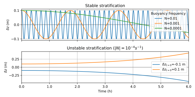
Static instability oscillations in a stably (top) and unstably (bottom) stratified fluid.

Exercises

Use the linear equation of state for seawater to demonstrate that the variations of density in the ocean are very small compared to the mean density. How large (in percent relative change) are these variations with respect to the changes in temperature, salinity, and pressure in the ocean?
Calculate the Brunt-Väisälä frequency for: (a) a typical mid-latitude thermocline with temperature decreasing from 20°C to 5°C over 500 m depth; (b) the deep ocean where potential temperature decreases from 4°C to 2°C over 2000 m depth. Assume constant salinity of 35 g/kg.

Summary

In this chapter, we covered:

The Boussinesq approximation, which assumes density variations are small compared to the mean density;
Decomposition of density and pressure into mean and perturbation components;
Static stability and its relationship to the vertical density gradient;
The Brunt-Väisälä frequency as a measure of stratification strength and the natural frequency of vertical oscillations in a stratified fluid.