Chapter 7

Shallow water systems

In this chapter we move away from the continuously stratified ocean and approximate it to a single layer of incompressible fluid that is also in hydrostatic balance. It turns out that this seemingly drastic approximation still allows the reduced equation set to reproduce many observed large scale oceanic and atmospheric phenomena. In other words, the shallow water equations may be about the simplest equation set thay yield relatively realistic and accurate atmospheric and oceanic flows. The simplicity of these equations allow for easier interpretation and testing of numerical implementations. For this reasons, many high-end weather, ocean, and climate models begin with a two-dimensional shallow water equations solver. In fact, this system of equations is the basis for some operational ocean prediction models, which are surprisingly accurate when applied to the nearshore and coastal ocean. We begin by introducing the key assumptions that allow the derivation of the shallow water equations, and after that we derive the general solutions to the equations.

Key assumptions

The name “shallow water” hints at the approximations that we will make about the flow:

Shallow: The vertical scale of the flow is much smaller than the horizontal scale. This doesn’t mean that there’s no vertical flow, only that the horizontal flow is the dominant one ( $u, v \gg w$ ).
Water: The flow is incompressible ( $\nabla \cdot \mathbf{u} = 0$ ).

As a consequence, our flow is also hydrostatic ( $dp/dz = -\rho g$ ). This approximation will show to be instrumental in allowing us to cast the horizontal pressure gradient in terms of the surface elevation only.

The flow can then be seen as a thin layer of fluid over a rigid bottom that may vary horizontally, and with a free surface that can freely move in the vertical in response to the horizontal flow, bottom topography, and incompressibility (Fig. 7.1). This layer of fluid may or may not be covered on top by another layer of fluid, with its own hydrostatic pressure imposed on the surface.

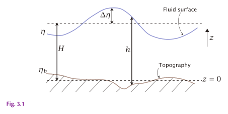
A shallow water system. is the thickness of a water column, its mean thickness, the height of the free surface and is th — Figure 7.1.
A shallow water system. $h$ is the thickness of a water column, $H$ its mean thickness, $\eta$ the height of the free surface and $\eta_b$ is the height of the lower, rigid surface above some arbitrary origin, typically chosen such that the average of $\eta_b$ is zero. $\Delta \eta$ is the deviation free surface height, so we have $\eta = \eta_b + h = H + \Delta \eta$ . This is Fig. 3.1 in AOFD (Vallis, 2017).

Shallow water equations

The shallow water equations consist of the momentum and the continuity equations. For 2-dimensional horizontal flow, the momentum equation can be expressed as a single equation in vector form, or as two scalar equations in $x$ and $y$ .

Momentum equation

We begin from the vector momentum equation with rotation:

\frac{d \mathbf{u}}{dt} + \mathbf{f} \times \mathbf{u} = - \frac{1}{\rho} \nabla p + \mathbf{g}

In the vertical component of this equation we will neglect the vertical acceleration to obtain the hydrostatic balance, as we did previously:

\frac{\partial p}{\partial z} = -\rho g

We can integrate the hydrostatic balance in $z$ to obtain the pressure as a function of height:

\int_{p(z)}^{p_\eta} dp = - \int_z^\eta \rho g \, dz

where $p_\eta$ is the pressure at $z = \eta$ . As this is the pressure at the free surface, it corresponds to the atmospheric pressure, if any. Rearranging the terms after integration yields:

p(z) = p_\eta + \rho g \eta - \rho g z

We will now apply a horizontal gradient to both sides and assume for simplicity that the horizontal gradient of $p_\eta$ is negligible compared to the other terms. In the context of the ocean surface, this would mean that the atmospheric pressure varies in the horizontal much less than the water elevation. This is almost always trivially satisfied. Further, taking that neither the density nor gravity vary in the horizontal, and noting that $z$ as a vertical coordinate cannot vary in the horizontal, we get:

\nabla p = \rho g \nabla \eta

Inserting Eq. 7.5 into Eq. 7.1, and taking $\nabla$ to be the horizontal divergence going forward, we get:

\frac{d \mathbf{u}}{dt} + \mathbf{f} \times \mathbf{u} = - g \nabla \eta

which is the horizontal shallow water momentum equation with rotation. Let’s now proceed to derive the shallow water continuity equation and complete the system of equations.

Continuity equation

An intuitive approach to deriving the shallow water continuity is to consider a column of fluid in a one-dimensional horizontal flow whose spatial variations would cause a change in the surface elevation of that column due to the incompressibility (Fig. 7.2). Although the bottom surface here is shown to be flat, recall from Fig. 7.1 that it doesn’t need to be, and the water column height $h$ comprises of the mean water depth $\overline{h}$ (as measured from the rigid bottom to the mean water level) plus the deviation of the free surface from the mean water level, $\eta$ :

h = \overline{h} + \eta

where the overline denotes a time average. This implies $\overline{\eta} = 0$ , by definition.

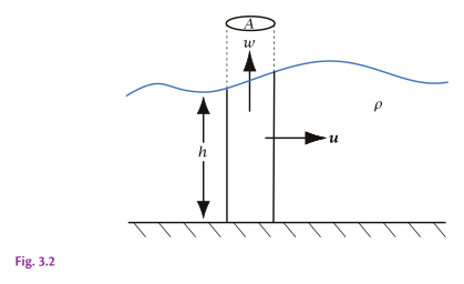
The mass budget for a column of area in a shallow water system. There is a non-zero vertical velocity at the top of the — Figure 7.2.
The mass budget for a column of area $A$ in a shallow water system. There is a non-zero vertical velocity at the top of the column if the mass convergence into the column is non-zero. This is Fig. 3.2 in AOFD (Vallis, 2017).

The difference between the amount of liquid flowing into and out of the column thus must be balanced by a change in the surface elevation of the column:

u_2 h_2 - u_1 h_1 = \frac{\partial \eta}{\partial t} \Delta x

Rearranging the terms leads to:

\frac{\partial \eta}{\partial t} = \frac{u_2 h_2 - u_1 h_1}{\Delta x} \approx \frac{\partial (u h)}{\partial x}

Generalized in vector form, this becomes the Eulerian form of the shallow water continuity equation:

\frac{\partial \eta}{\partial t} + \nabla \cdot (h \mathbf{u}) = 0

which states that the local change in surface elevation is governed by the divergence of the horizontal flow through the water column. Since a gradient of $h$ can capture either the surface elevation or the mean water depth gradients, this equation is valid for both flat and varying bottom topography.

How about the Lagrangian form of the shallow water continuity? From Eq. (7.10), expand the divergence term and the water colum height $h$ , and express the rate of change of $\eta$ as a total derivative to get:

\frac{d\eta}{dt} - \mathbf{u} \cdot \nabla \eta + (\overline{h} + \eta) \nabla \cdot \mathbf{u} + \mathbf{u} \cdot \nabla (\overline{h} + \eta) = 0

\frac{d\eta}{dt} + h \nabla \cdot \mathbf{u} + \mathbf{u} \cdot \nabla \overline{h} = 0

Now, recognize that the advective component of the bottom topography gradient $\mathbf{u} \cdot \nabla \overline{h}$ must be the Lagrangian rate of change of the mean water depth, $d\overline{h}/dt$ , because the bottom topography is fixed in time and the only way for a fluid parcel to experience a change in mean water depth is to move horizontally. Thus, we can write:

\frac{d\eta}{dt} + h \nabla \cdot \mathbf{u} + \frac{d \overline{h}}{dt} = 0

or simply:

\frac{dh}{dt} + h \nabla \cdot \mathbf{u} = 0

The Lagrangian form of the shallow water continuity can thus be expressed either in terms of the total water column height $h$ , in which case it takes the familiar form, or in terms of the surface elevation $\eta$ , in which case it has an additional term that accounts for the bottom topography gradient. To get the Eulerian form from here, we first need to recognize that $d\eta/dt = dh/dt$ because $h = \overline{h} + \eta$ , where $\overline{h}$ is the mean water depth. Then, expanding the Lagrangian derivative, we recover Eq. 7.10.

The complete equation set

The momentum and continuity equations that we derived above form the complete set of shallow water equations. In vector form, they are:

\frac{d \mathbf{u}}{dt} + \mathbf{f} \times \mathbf{u} = - g \nabla \eta

\frac{\partial \eta}{\partial t} + \nabla \cdot (h \mathbf{u}) = 0

And in scalar form, in two dimensions:

\frac{\partial u}{\partial t} + u \frac{\partial u}{\partial x} + v \frac{\partial u}{\partial y} - f v = -g \frac{\partial \eta}{\partial x}

\frac{\partial v}{\partial t} + u \frac{\partial v}{\partial x} + v \frac{\partial v}{\partial y} + f u = -g \frac{\partial \eta}{\partial y}

\frac{\partial \eta}{\partial t} + \frac{\partial (hu)}{\partial x} + \frac{\partial (hv)}{\partial y} = 0

which closes our system of equations. In two dimensions, we thus have three equations for the three unknown variables $u$ , $v$ , and $\eta$ . The flow is inviscid (no friction) but nonlinear (advective term $\mathbf{u} \cdot \nabla \mathbf{u}$ is present), so this system of equations allows for turbulence but does not dissipate energy. Also, notice that the Coriolis force is present but has seamlessly percolated from the starting equation without breaking any of the assumptions. Thus, to consider shallow water systems in a non-rotating frame, simply drop the Coriolis terms.

We now proceed to further simplify this equation set to derive a general solution for the shallow water equations.

Poincaré waves

As we proceed to derive a solution to the equations (7.17-7.19), notice that the nonlinear terms get in the way of an analytical solution. To work around this, we will assume a flat bottom $H$ such that:

h(x, y, t) = H + \eta(x, y, t)

Insert it into Eqs. (7.15) and (7.16) to get:

\frac{\partial \mathbf{u}}{\partial t} + \mathbf{u} \cdot \nabla \mathbf{u} + \mathbf{f} \times \mathbf{u} = - g \nabla \left( H + \eta \right)

\frac{\partial \eta}{\partial t} + \nabla \cdot \left[ (H + \eta) \mathbf{u} \right] = 0

Although we do not require that the perturbations on their own are small enough to neglect, the products of two perturbations are assumed to be. This allows us to linearize the equations and obtain:

\frac{\partial \mathbf{u}}{\partial t} + \mathbf{f} \times \mathbf{u} + g \nabla \eta = 0

\frac{\partial \eta}{\partial t} + H \nabla \cdot \mathbf{u} = 0

Or, in scalar form:

\frac{\partial u}{\partial t} - f v + g \frac{\partial \eta}{\partial x} = 0

\frac{\partial v}{\partial t} + f u + g \frac{\partial \eta}{\partial y} = 0

\frac{\partial \eta}{\partial t} + H \frac{\partial u}{\partial x} + H \frac{\partial v}{\partial y} = 0

This is a linear system of three equations with three unknowns, $u$ , $v$ , and $\eta$ . To solve it, we will look for wave-like solutions:

(u, v, \eta) = (\widehat{u}, \widehat{v}, \widehat{\eta}) e^{i(kx + ly - \omega t)}

where $\widehat{u}$ , $\widehat{v}$ , and $\widehat{\eta}$ are the wave amplitudes, $k$ and $l$ are the zonal and meridional wavenumbers, respectively, and $\omega$ is the angular frequency. It is now worthwhile to pause and discuss what is a wave and how would we get the idea to assume a wave form for the solution. A wave is a disturbance in the medium that propagates through it with some characteristic speed. In our case, the wave is periodic, meaning that the disturbance repeats itself in space and time. That’s the meaning of the phase function $\phi = kx + ly - \omega t$ in the exponent: it determines where in the wave cycle we are at a given point in space and time. The assumption that the solution to the equations is a periodic wave is informed by the fact that derivatives of periodic functions are also periodic, and this will allow the wave form ( $e^{i\phi}$ ) to factor out of the equations, leaving only the amplitudes and the wave parameters ( $k$ , $l$ , $\omega$ ) to determine the solution.

Now, insert the wave form into Eqs. (7.25-7.27) to get:

- i \omega \widehat{u} - f \widehat{v} + i g k \widehat{\eta} = 0

- i \omega \widehat{v} + f \widehat{u} + i g l \widehat{\eta} = 0

- i \omega \widehat{\eta} + i H k \widehat{u} + i H l \widehat{v} = 0

or, in matrix form:

\begin{bmatrix} - i \omega & - f & i g k \\ f & - i \omega & i g l \\ i H k & i H l & - i \omega \end{bmatrix} \begin{bmatrix} \widehat{u} \\ \widehat{v} \\ \widehat{\eta} \end{bmatrix} = 0

The solution to this system requires that the determinant of the matrix be zero, which yields:

\omega[\omega^2 - f^2 - gH(k^2 + l^2)] = 0

A trivial solution to this equation is $\omega = 0$ , which corresponds to an unperturbed, constant flow. The other, non-trivial solution is the dispersion relation for shallow water gravity waves in a rotating frame:

\omega = \sqrt{f^2 + gH(k^2 + l^2)}

This dispersion relationship connects the frequency to the wavenumber, and we see that it scales with the Coriolis frequency $f$ and the gravity wave phase speed $\sqrt{gH}$ . This general solution is called a Poincaré wave, a surface gravity wave with effects of rotation. Poincaré waves are also commonly referred to as inertial-gravity waves. Increasing the Coriolis parameter $f$ while keeping the other parameters fixed increases the frequency of the waves by enhancing the rotation. Similarly, increasing the gravitational acceleration $g$ or the mean water depth $H$ increases the frequency of the waves by enhancing the gravity wave phase speed. Notice also that the frequency $\omega$ scales linearly with the wavenumber $k^2 + l^2$ , their ratio $\omega / (k^2 + l^2)$ being the phase speed of the wave:

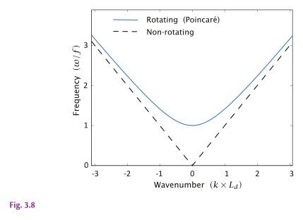
c_p = \frac{\omega}{\sqrt{k^2 + l^2}} = \sqrt{\frac{f^2}{k^2 + l^2} + gH}

Figure 7.3.
Dispersion relation for Poincaré waves and non-rotating shallow water waves. Frequency is scaled by the Coriolis frequency $f$ , and wavenumber by the inverse deformation radius $\sqrt{gH}/f$ . For small wavenumbers the frequency of the Poincaré waves is approximately $f$ , and for high wavenumbers is asymptotes to that of non-rotating waves. This is Fig. 3.8 in AOFD (Vallis, 2017).

As there are two independent parameters in Eq. 7.34 that originate from different terms in the shallow water equations, we can turn the knobs on each to explore some limiting cases of the general solution.

Short gravity waves

In the case of short gravity waves, the pressure gradient terms (and thus, gravity) dominate the Coriolis term (rotation):

gH(k^2 + l^2) \gg f^2

In this case, the dispersion relation simplifies to:

\omega = \sqrt{gH(k^2 + l^2)}

which is the dispersion relation for (non-rotating) shallow water gravity waves. Notice, however, that we don’t require there to be no rotation at all to obtain the non-rotating gravity waves. Rather, we simply require that the waves are so short (high wavenumber) that the Coriolis force is negligible compared to the gravity force. The phase speed of these waves, that is, the speed at which they propagate, is:

C_p = \frac{\omega}{k} = \sqrt{g h}

Real-life examples of this solution include tsunamis, wind-generated swell waves on the ocean surface, or small ripples that propagate radially outward when throwing a stone into a pond.

Inertial oscillations

If the wavenumber is so small (large wavelength) that the gravity term can be neglected in favor of the Coriolis term, we recover a class of motion that we explored earlier, the inertial oscillations. In this case, the rotation dominates over the gravity:

f^2 \gg gH(k^2 + l^2)

and the dispersion relation simplifies to:

\omega = f

which corresponds to a circular motion with the frequency that exactly equals the Coriolis frequency (because $(u, v) = (\widehat{u}, \widehat{v}) e^{- i f t}$ ). Recall that we already explored this solution by dropping the pressure gradient terms in the rotating momentum equations back in Section Inertial oscillations. Here, it comes out as a limiting case from the general solution which we couldn’t obtain prior to the shallow water approximations and linearization.

Kelvin waves

A special case of the general solution that is particularly relevant to the atmospheric and oceanic dynamics is that of a linearized shallow water flow that is bounded on one side by a solid boundary, such as a coastline. The resulting solution is a special class of gravity waves called Kelvin waves, which propagate as a shallow water gravity wave along the solid boundary and whose propagation direction, as well as the perturbation scale in the direction away from the boundary, are governed by the planetary rotation rate. Kelvin waves appear in both the atmosphere and the ocean.

To derive the Kelvin waves, we start from the linearized shallow water equations (where we drop the primes for brevity):

\frac{\partial u}{\partial t} - f v = - g \frac{\partial \eta}{\partial x}

\frac{\partial v}{\partial t} + f u = - g \frac{\partial \eta}{\partial y}

\frac{\partial \eta}{\partial t} + H \left( \frac{\partial u}{\partial x} + \frac{\partial v}{\partial y} \right) = 0

Now, suppose that our solid boundary is along the $x$ -axis at $y = 0$ , which allows us to neglect the meridional flow ( $v=0$ ):

\frac{\partial u}{\partial t} = - g \frac{\partial \eta}{\partial x}

f u = - g \frac{\partial \eta}{\partial y}

\frac{\partial \eta}{\partial t} + H \frac{\partial u}{\partial x} = 0

Differentiate Eq. 7.44 with respect to time and Eq. 7.46 with respect to $x$ , and combine them to get:

\frac{\partial^2 u}{\partial t^2} - gH \frac{\partial^2 u}{\partial x^2} = 0

which is the standard wave equation, whose solution is a wave that propagates with the phase speed $c = \sqrt{gH}$ . We will thus assume a wave-like solution for $u$ , like we did for the Poincaré waves in Section Poincaré waves. However, since we now have a solid boundary at $y = 0$ , we should also assume that the solution should vary in the $y$ direction (because it must be zero at the boundary, and non-zero elsewhere). The general solution for $u$ may be:

u = \widehat{u}(y) e^{i(x - c t)}

Notice that we have now assumed the wave phase in the form of $(x - c t)$ , as opposed to $(kx - \omega t)$ . This is because we already know the phase speed $c$ , as well as for mathematical convenience; the two wave forms are otherwise equivalent. As for the elevation $\eta$ , insert Eq. 7.48 into Eq. 7.46 to get:

\eta = \sqrt{\frac{H}{g}} \widehat{u}(y) e^{i(x - c t)}

We still need to solve for $\widehat{u}(y)$ , so we look for the equation that has a derivative with respect to $y$ . So, insert Eqs. 7.48 and 7.49 into Eq. 7.45 to get:

f \widehat{u}(y) = - \sqrt{\frac{H}{g}} \frac{\partial \widehat{u}(y)}{\partial y}

which integrates to:

\widehat{u}(y) = \widehat{u}_0 e^{-\frac{fy}{\sqrt{gH}}} = \widehat{u}_0 e^{-\frac{y}{L_d}}

where

L_d = \frac{\sqrt{gH}}{f}

is the Rossby radius of deformation , which is the length scale at which planetary rotation becomes important relative to the effects of gravity (or buoyancy, in stratified flows). The complete solutions for the shallow water Kelvin waves are then:

u = \widehat{u}_0 e^{-\frac{y}{L_d}} e^{i(x - c t)}

\eta = \sqrt{\frac{H}{g}} \widehat{u}_0 e^{-\frac{y}{L_d}} e^{i(x - c t)}

which is a wave in the direction along the rigid boundary ( $y=0$ ) whose amplitude decays exponentially away from the boundary, with a decay scale equal to the Rossby radius of deformation $L_d$ . The choice of the orientation of the rigid boundary at $y=0$ is arbitrary; if we had chosen the boundary at $x=0$ , the solution would be a wave propagating in the $y$ direction and decaying in the $x$ direction. If it were oriented at some arbitrary angle between $x$ and $y$ axes, the solution would be a 2-d wave in $x$ and $y$ and with their respective wavenumbers controlling the phase speed in each direction.

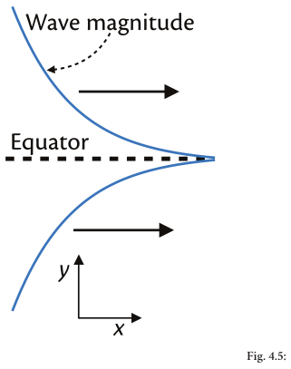
Kelvin waves propagating eastward along the equator and decaying rapidly away to either side. This is Fig. 4.5 in Vallis (EAOD).

Conservative properties

We now look at some conservative properties of the shallow water equations, namely the potential vorticity conservation and the conservation of energy. The former is a material conservative property, meaning that it is conserved along a fluid parcel as it moves and deforms. The latter is a volume-integrated conservative property, meaning that it is conserved in a control volume as the fluid evolves in time. The conservation of potential vorticity yields some interesting emerging properties of the flow, such as the vortex stretching due to the change in the fluid depth, and the planetary waves due to the meridional variation of the planetary vorticity (Coriolis parameter $f$ ).

Potential vorticity

Potential vorticity (PV) describes the rate of rotation of a fluid parcel scaled by the fluid depth. It is a material property, meaning that it is conserved along a fluid parcel as it moves and deforms. In shallow water systems, the conservation of potential vorticity allows us to predict how an eddy’s spin may change as it moves into shallower or deeper water, or if it moves north or south on a rotating planet.

First, some definitions as this is the first place that we encounter vorticity. Vorticity is a measure of the local rotation of a fluid parcel, and is defined as the curl of the velocity field:

\boldsymbol{\omega} = \nabla \times \mathbf{u} = \begin{bmatrix} \mathbf{i} & \mathbf{j} & \mathbf{k} \\ \frac{\partial}{\partial x} & \frac{\partial}{\partial y} & \frac{\partial}{\partial z} \\ u & v & w \end{bmatrix} = \begin{bmatrix} \frac{\partial w}{\partial y} - \frac{\partial v}{\partial z} \\ \frac{\partial u}{\partial z} - \frac{\partial w}{\partial x} \\ \frac{\partial v}{\partial x} - \frac{\partial u}{\partial y} \end{bmatrix}

In largely 2-d flows, the vertical component of vorticity is the most relevant, and hereon we will use a separate symbol for it:

\zeta = \frac{\partial v}{\partial x} - \frac{\partial u}{\partial y}

Vorticity of a flow is a complementary property to its divergence. A flow can be either rotational (non-zero vorticity) or irrotational (zero vorticity), and either divergent (non-zero divergence) or non-divergent (zero divergence). It can be both rotational and divergent, or neither. However, that they are complementary (and in a way, orthogonal) properties of the flow can be shown mathematically by the fact that the divergence of vorticity is always zero:

\nabla \cdot \nabla \times \mathbf{u} = 0

This means simply that once you extract the vorticity from a flow by taking $\nabla \times \mathbf{u}$ , any divergence that may have been present in the flow is left behind.

Back to our potential vorticity conservation derivation, start from the momentum equation with effects of rotation:

\frac{\partial \mathbf{u}}{\partial t} + \mathbf{u} \cdot \nabla \mathbf{u} + \mathbf{f} \times \mathbf{u} = - g \nabla \eta

We will rely on the following vector identity to rewrite the advective term:

\mathbf{u} \cdot \nabla \mathbf{u} = \frac{1}{2} \nabla (\mathbf{u}^2) - \mathbf{u} \times (\nabla \times \mathbf{u})

and recognize $\nabla \times \mathbf{u} = \boldsymbol{\omega}$ as the vorticity to rewrite the above as:

\frac{\partial \mathbf{u}}{\partial t} + \left(\boldsymbol{\omega} + \mathbf{f}\right) \times \mathbf{u} = - g \nabla \left(\eta + \frac{1}{2} \mathbf{u}^2 \right)

Take a curl of this equation to get:

\frac{\partial (\nabla \times \mathbf{u})}{\partial t} + \nabla \times \left[(\boldsymbol{\omega} + \mathbf{f}) \times \mathbf{u}\right] = - g \nabla \times \nabla \left(\eta + \frac{1}{2} \mathbf{u}^2 \right)

Since the curl of a gradient is always zero, the right-hand side vanishes, and we are left with:

\frac{\partial \boldsymbol{\omega}}{\partial t} + \nabla \times \left[(\boldsymbol{\omega} + \mathbf{f}) \times \mathbf{u}\right] = 0

Next, we use the vector triple product identity:

\nabla \times \boldsymbol{\omega} \times \mathbf{u} = (\mathbf{u} \cdot \nabla) \boldsymbol{\omega} - (\boldsymbol{\omega} \cdot \nabla) \mathbf{u} + \boldsymbol{\omega} \nabla \cdot \mathbf{u} - \mathbf{u} \nabla \cdot \boldsymbol{\omega}

Since vorticity must be divergence free ( $\nabla \cdot \boldsymbol{\omega} = 0$ ), and it’s perpendicular to the velocity vector ( $\boldsymbol{\omega} \cdot \mathbf{u} = 0$ ), the second and the fourth terms vanish. Define the vertical component of the vorticity to be:

\zeta = \mathbf{k} \cdot \boldsymbol{\omega}

to get:

\frac{\partial \zeta}{\partial t} + \left(\mathbf{u} \cdot \nabla \right) \left(\zeta + f\right) = - \left(\zeta + f\right) \nabla \cdot \mathbf{u}

Recall the continuity equation:

\frac{dh}{dt} = -h \nabla \cdot \mathbf{u}

Multiply both sides by $(\zeta + f)$ to write:

\frac{dh}{dt} \frac{\zeta + f}{h} = - \left(\zeta + f\right) \nabla \cdot \mathbf{u}

\frac{d(\zeta + f)}{dt} = \frac{\zeta + f}{h} \frac{dh}{dt}

Then, notice that:

\frac{d}{dt} \left( \frac{\zeta}{h} \right) = \frac{1}{h} \frac{d\zeta}{dt} + \zeta \frac{d}{dt} \left( \frac{1}{h} \right) = \frac{1}{h} \frac{d\zeta}{dt} - \frac{\zeta}{h^2} \frac{dh}{dt} = \frac{1}{h} \left( \frac{d\zeta}{dt} - \frac{\zeta}{h} \frac{dh}{dt} \right)

which leads to:

\frac{d}{dt} \left( \frac{\zeta + f}{h} \right) = 0

where $(\zeta + f)/h$ is the potential vorticity, and Eq. 7.70 is the conservation of potential vorticity.

Let’s consider some implications of it. First, without planetary rotation ( $f = 0$ ), potential vorticity is $\zeta/h$ . Imagine a parcel of fluid with some vorticity $\zeta$ (for example, a small eddy). The eddy propagates zonally over a seamount such that the mean water depth gradually decreases. As the eddy enters progressively shallower water, its vorticity must increase so that the potential vorticity is conserved. An cold eddy (with $\zeta > 0$ ) will thus rotate more rapidly (cyclonically, or counter-clockwise in the Northern Hemisphere) as it approaches the tip of the seamount where the water is shallowest, and then decrease again as it moves away from the tip of the seamount into deeper water. Similarly, a warm eddy (with $\zeta < 0$ ) will weaken its anticyclonic (clockwise) rotation as it moves toward the tip of the seamount, and then strengthen it again as it moves away from the tip of the seamount into deeper water. Another consequence of the conservation of potential vorticity is that on a $\beta$ -plane, or more generally, a rotating sphere, where the Coriolis parameter $f$ varies with latitude, the vorticity of a parcel will adjust to meridional displacements and changes in $f$ to conserve potential vorticity. The latter mechanism yields the so-called Rossby waves, a key feature of mid-latitude weather dynamics.

Energy

Start from the definitions of potential and kinetic energy:

PE = \int_0^h \rho g z\ dz = \frac{1}{2} \rho g h^2

KE = \int_0^h \frac{1}{2} \rho \mathbf{u}^2\ dz = \frac{1}{2} \rho \mathbf{u}^2 h

The total energy is the sum of potential and kinetic energy:

E = PE + KE = \frac{1}{2} \rho g h^2 + \frac{1}{2} \rho \mathbf{u}^2 h

Let’s now proceed to derive the PE and KE equations for the shallow water systems. Recall the shallow water continuity equation:

\frac{dh}{dt} + h \nabla \cdot \mathbf{u} = 0

Multiply it by $gh$ to get:

\frac{d}{dt} \left( \frac{gh^2}{2} \right) + gh^2 \nabla \cdot \mathbf{u} = 0

Expand the Lagrangian derivative:

\frac{\partial}{\partial t} \left( \frac{gh^2}{2} \right) + \mathbf{u} \cdot \nabla \left( \frac{gh^2}{2} \right) + gh^2 \nabla \cdot \mathbf{u} = 0

Then, we borrow a half of the third term to combine it with the second term:

\frac{\partial}{\partial t} \left( \frac{gh^2}{2} \right) + \nabla \left( \mathbf{u} \frac{gh^2}{2} \right) + \frac{gh^2}{2} \nabla \cdot \mathbf{u} = 0

which is the equation for the evolution of potential energy. Note that the density $\rho$ is assumed constant and is omitted here for brevity.

Next, recall the momentum equation, assuming uniform mean water depth for simplicity:

\frac{d\mathbf{u}}{dt} = - g \nabla h

Multiply this by $\mathbf{u}$ and re-arrange to get:

\mathbf{u} h \frac{d\mathbf{u}}{dt} + g\mathbf{u}h\nabla h = 0

\frac{d}{dt} \left( \frac{h \mathbf{u}^2}{2} \right) - \frac{\mathbf{u}^2}{2} \frac{dh}{dt} + g\mathbf{u}\nabla \left(\frac{h^2}{2}\right) = 0

Recall the shallow water continuity to write:

\frac{d}{dt} \left( \frac{h \mathbf{u}^2}{2} \right) + \frac{h\mathbf{u}^2}{2} \nabla \cdot \mathbf{u} + g\mathbf{u}\nabla \left(\frac{h^2}{2}\right) = 0

Expand the Lagrangian derivative:

\frac{\partial}{\partial t} \left( \frac{h \mathbf{u}^2}{2} \right) + \mathbf{u} \cdot \nabla \left( \frac{h \mathbf{u}^2}{2} \right) + \frac{h\mathbf{u}^2}{2} \nabla \cdot \mathbf{u} + g\mathbf{u}\nabla \left(\frac{h^2}{2}\right) = 0

and combine the second and third terms to write:

\frac{\partial}{\partial t} \left( \frac{h \mathbf{u}^2}{2} \right) + \nabla \cdot \left( \mathbf{u} \frac{h \mathbf{u}^2}{2} \right) + g\mathbf{u}\nabla \left(\frac{h^2}{2}\right) = 0

which is the equation for the evolution of kinetic energy.

Now, combine Eqs. 7.77 and 7.83 to get:

\frac{\partial}{\partial t} \frac{1}{2} \left(h\mathbf{u}^2 + gh^2\right) + \nabla \cdot \left[ \mathbf{u} \left( \frac{1}{2} h\mathbf{u}^2 + gh^2\right) \right] = 0

which is the conservation of total energy $E = PE + KE$ , and $\mathbf{F} = \mathbf{u} \left( \frac{1}{2} h\mathbf{u}^2 + gh^2\right)$ is the energy flux such that we can write:

\frac{\partial E}{\partial t} + \nabla \cdot \mathbf{F} = 0

The total energy of the system $E$ is thus conserved and entirely governed by the divergence of the energy flux $\mathbf{F}$ .

Rossby waves

One emerging pattern from the conservation of potential vorticity arises if the planetary vorticity $f$ is allowed to vary with latitude. This is true on a sphere where $f = 2 \Omega \sin(\theta)$ , or on a $\beta$ -plane where $f = f_0 + \beta y$ . This pattern is called Rossby waves (also called planetary waves) and is among the most important classes of motions in both the ocean and the atmosphere.

To derive the solution for Rossby waves, we start from the shallow-water potential vorticity conservation equation:

\frac{d}{dt} \left( \frac{\zeta + f}{h} \right) = 0

To simplify the derivation, we will assume a flat bottom so that

\frac{d(\zeta + f)}{dt} = 0

Expand the Lagrangian derivative to get:

\frac{\partial \zeta}{\partial t} + \mathbf{u} \cdot \nabla \zeta + v \beta = 0

which is the potential vorticity conservation equation on a $\beta$ -plane.

We still have only one equation with two unknowns, albeit two related unknowns (relative vorticity $\zeta$ and velocity $\mathbf{u}$ ). We somehow need to reduce them to one unknown variable. One approach is to introduce a streamfunction $\psi$ such that:

(u, v) = \left( - \frac{\partial \psi}{\partial y}, \frac{\partial \psi}{\partial x} \right)

We can then express the relative vorticity in terms of the streamfunction as:

\zeta = \frac{\partial v}{\partial x} - \frac{\partial u}{\partial y} = \frac{\partial^2 \psi}{\partial x^2} + \frac{\partial^2 \psi}{\partial y^2} = \nabla^2 \psi

Then, insert Eqs. 7.89 and 7.90 into Eq. 7.88, and linearize $u$ in the advective term such that the relative vorticity is only advected by the steady zonal flow $U$ :

\frac{\partial}{\partial t} \nabla^2 \psi + U \frac{\partial}{\partial x} \nabla^2 \psi + \beta \frac{\partial \psi}{\partial x} = 0

which is the potential vorticity equation on a $\beta$ -plane in terms of the streamfunction.

As before, assume a wave-like solution but this time for the streamfunction:

\psi = \widehat{\psi} e^{i(kx - \omega t)}

and insert it into Eq. 7.91 to get:

k \left( k\omega - Uk^2 + \beta \right) = 0

As before, $k = 0$ is a trivial and non-interesting solution, as it corresponds to there being no wave at all. For the non-trivial solution, rearranging the terms to get the equation for frequency yields the dispersion relation for Rossby waves:

\omega = U k - \frac{\beta}{k}

The phase speed of Rossby waves is:

c_p = \frac{\omega}{k} = U - \frac{\beta}{k^2}

and their group speed, that is, the speed at which the wave energy propagates, is:

c_g = \frac{\partial\omega}{\partial k} = U + \frac{\beta}{k^2}

Like in the case of the Poincaré waves, the frequency (or the phase speed) of Rossby waves do not depend on the wave amplitude ( $\widehat{\psi}$ ), which is a consequence of the linearization. Instead, they depend on the wavenumber $k$ (inverse wave length), the magnitude of the steady zonal flow $U$ , and the meridional Coriolis gradient $\beta$ . $U$ is here simply a linear Doppler shift term, and does not affect the wave’s intrinsic properties; it merely translates it. The second term, $-\beta/k$ , is the intrinsic frequency of Rossby waves, which is always negative because $\beta = 2\Omega \cos{\theta} > 0$ . This means that Rossby waves always propagate westward relative to the mean flow ( $c_p - U < 0$ ). Further, depending on their scale and the magnitude of the zonal flow, their phase can be stationary ( $c_p = 0$ ) or even eastward propagating ( $c_p > 0$ ). However, their intrinsic group speed is always positive ( $c_g > 0$ ), and thus, even in the case of no background zonal flow ( $U=0$ ), their energy propagates eastward.

Figure 7.5.
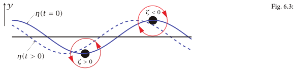
A two-dimensional (x-y) Rossby wave. An initial disturbance displaces a material line at constant latitude (the straight horizontal line) to the solid line marked $\eta(t=0)$ . Conservation of potential vorticity, $\zeta + \beta y$ , leads to the production of relative vorticity, $\zeta$ , as shown. The associated velocity field (arrows on the circles) then advects the fluid parcels, and the material line evolves into the dashed line with the phase propagating westward. This is Fig. 6.3 in Vallis (EAOD).

Rossby waves are named after Carl-Gustaf Rossby, an American meteorologist of Swedish origin, who first identified these waves while studying large scale flow in the atmosphere in the 1930s. The Carl-Gustaf Rossby Research Medal is the highest award in atmospheric sciences, has been awarded by the American Meteorological Society since 1951.

Exercises

Assuming shallow water approximation and mid-latitudes, quantify the relative importance of planetary rotation in the flow for (a) wind-generated swell waves, (b) a submesoscale eddy, (c) Gulf Stream, and (d) a synoptic-scale cyclone in the atmosphere.
Consider characteristic mid-latitude flows on Earth, Jupiter, and Titan. At what spatial scales does the gravity play equal role as the rotation? Assume the shallow water dispersion relationship for your analysis.
An ocean eddy with initial relative vorticity $\zeta_0$ begins its journey northward at 30 $^\circ$ N and depth of 2000 m and travels with the mean flow to 40 $^\circ$ N and depth of 1000 m. Assuming the potential vorticity of the eddy is conserved, calculate the its final relative vorticity.
Find the expression for the wavenumber of a stationary Rossby wave as a function of latitude and the mean zonal flow. Then, calculate the wavelength of a stationary Rossby wave at 45 $^\circ$ N, in a mean zonal flow of 10 m/s.

Summary

In this chapter, we covered:

The shallow water equations as a simplified model for large-scale ocean and atmospheric flows;
Key assumptions of the shallow water system: horizontal scales much larger than vertical scales, incompressible flow, and hydrostatic balance;
Conservation of potential vorticity and its role in generating relative vorticity as fluid parcels move meridionally.
Rossby waves - westward propagating planetary waves that arise from the variation of the Coriolis parameter with latitude;
The dispersion relationship and phase speed of Rossby waves;