Chapter 8

Turbulence

Turbulence is the nonlinear and chaotic fluid motion that occurs when a fluid is driven by sufficiently strong forces. It is characterized by large fluctuations in time and space and over a broad range of scales. Fluid elements with high vorticity of either sign move and interact with each other, transferring energy and vorticity across scales. In this chapter, we investigate turbulence from the point of view of the governing equations of fluid motion. The key pursuit of fluid mechanics of turbulence is to predict the evolution of mean flow while accounting for the effects of turbulence. We begin by introducing the Reynolds decomposition, a fundamental tool in the study of turbulence that allows separating the flow into a slowly evolving mean part and a rapidly fluctuating turbulent part. Applying the Reynolds decomposition to the Navier-Stokes equation leads to the Reynolds-averaged Navier-Stokes (RANS) equation, which is the prognostic equation for the mean flow. We will discuss the so-called closure problem of turbulence, which is the challenge of representing the effects of the smallest scales on the larger scales. Using the RANS equation, we will derive the turbulent kinetic energy budget equation, and investigate the turbulent cascade in both 2D and 3D flows. The new understanding from this chapter will allow us to study the boundary layers in the atmosphere and the ocean alike.

Reynolds decomposition

Before we apply any scale separation to the Navier-Stokes equation, let’s first define the Reynolds decomposition that breaks the flow $u$ into the time-mean and fluctuating parts:

\mathbf{u}(x, t) = \overline{\mathbf{u}}(x) + \mathbf{u}'(x, t)

The time average is defined as:

\overline{\mathbf{u}}(x) = \frac{1}{T} \int_{t_0}^{t_0 + T} \mathbf{u}(x, t)\ dt

Already we need to make a choice about the averaging time $T$ . This choice is arbitrary and usually driven by the practical limitations of the problem. Typical weather and ocean ciculation models take $T$ to be on the order of seconds (for a regional weather prediction model) to minutes (for a mesoscale ocean circulation model). The turbulence itself operates on much shorter time scales, typically on the order of milliseconds to seconds for atmospheric and oceanic flows.

Let’s look at some mathematical properties of the Reynolds decomposition. If we take the time average of 8.1, we get:

\overline{\mathbf{u}(x, t)} = \overline{\overline{\mathbf{u}}(x) + \mathbf{u}'(x, t)}

which leads to:

\overline{\mathbf{u}'(x, t)} = 0

Notice that we specifically average over time, not space, which allows the mean flow to vary in space. We could have as easily defined the average in 8.1 to be over a spatial domain (or any other dimension), and those are indeed useful for other things.

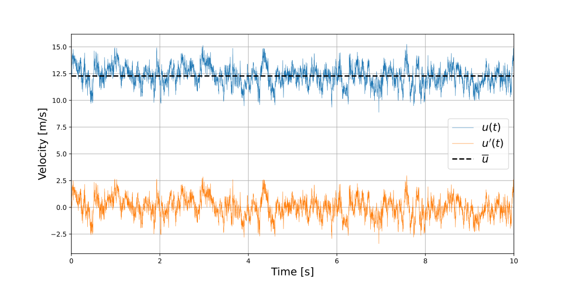
An 10-second example sequence of horizontal velocity (blue) measured at 1000 Hz using a Constant Temperature Anemometer — Figure 8.1.
An 10-second example sequence of horizontal velocity $u$ (blue) measured at 1000 Hz using a Constant Temperature Anemometer in the Air-Sea Interaction Saltwater Tank (ASIST) at the University of Miami. Dashed black line shows the time-mean velocity $\overline{u}$ calculated over the 10-second interval, and the orange line shows the fluctuating part.

The averaging operation is commutative with respect to derivatives and integrals, over space or time alike:

\overline{\frac{\partial \mathbf{u}}{\partial t}} = \frac{\partial \overline{\mathbf{u}}}{\partial t}

\overline{\nabla \cdot \mathbf{u}} = \nabla \cdot \overline{\mathbf{u}}

\overline{\int \mathbf{u} dt} = \int \overline{\mathbf{u}} dt

Although here we have defined the Reynolds decomposition using the velocity field, it can be applied to any field variable, vector or scalar alike.

If the flow is incompressible ( $\nabla \cdot \mathbf{u} = 0$ ), then the mean flow is incompressible as well:

\nabla \cdot \overline{\mathbf{u}} = 0

and by definition the fluctuating field must also be divergence-free:

\nabla \cdot \mathbf{u} = \nabla \cdot (\overline{\mathbf{u}} + \mathbf{u}') = \nabla \cdot \overline{\mathbf{u}} + \nabla \cdot \mathbf{u}' = 0

\nabla \cdot \mathbf{u}' = 0

An example of the Reynolds decomposition applied to a measured turbulent velocity time series is shown in Fig. 8.1.

Reynolds-Averaged Navier-Stokes (RANS) equation

We seek the governing equations for the mean flow that include the effects of the fluctuating field (turbulence). To do that, let’s apply the Reynolds decomposition to the Navier-Stokes equation and take the time average of the resulting equation. We begin by writing out Eq. 4.36 without the body forces, for simplicity (as the body forces won’t be affected by the Reynolds decomposition):

\frac{\partial \mathbf{u}}{\partial t} + \mathbf{u} \cdot \nabla \mathbf{u} = - \frac{1}{\rho} \nabla p + \nu \nabla^2 \mathbf{u}

It’s at this time useful to re-cast this equation in the momentum-conservative form that is prognostic for the momentum $\rho \mathbf{u}$ rather than just the velocity $\mathbf{u}$ . To do that, multiply Eq. 8.11 by $\rho$ to get:

\rho \frac{\partial \mathbf{u}}{\partial t} + \rho \mathbf{u} \cdot \nabla \mathbf{u} = - \nabla p + \mu \nabla^2 \mathbf{u}

while recalling that the kinematic viscosity $\nu$ is defined as $\nu = \mu / \rho$ . Now, we will use the Eulerian form of the continuity equation (Eq. 4.4) to reframe the left-hand side of Eq. 8.12 in terms of the momentum $\rho \mathbf{u}$ :

\begin{split} \rho \frac{\partial \mathbf{u}}{\partial t} + \rho \mathbf{u} \cdot \nabla \mathbf{u} \\ = \frac{\partial (\rho \mathbf{u})}{\partial t} - \mathbf{u} \frac{\partial \rho}{\partial t} + \rho \mathbf{u} \cdot \nabla \mathbf{u} \\ = \frac{\partial (\rho \mathbf{u})}{\partial t} + \mathbf{u} \nabla \cdot (\rho \mathbf{u}) + \rho \mathbf{u} \cdot \nabla \mathbf{u} \\ = \frac{\partial (\rho \mathbf{u})}{\partial t} + \nabla \cdot (\rho \mathbf{u} \mathbf{u}) \end{split}

Take a moment to notice and understand that $\mathbf{u}\mathbf{u}$ in the last term is a second-order tensor rather than a scalar $\mathbf{u} \cdot \mathbf{u} = \mathbf{u}^2$ . Its physical interpretation as advective flux still remains as before; the only difference is that the advective velocity is now inside the derivative.

Back to our momentum equation (Eq. 8.12), we can now write it as:

\frac{\partial (\rho \mathbf{u})}{\partial t} + \nabla \cdot (\rho \mathbf{u} \mathbf{u}) = - \nabla p + \mu \nabla^2 \mathbf{u}

and in case of incompressible flows ( $\nabla \cdot \mathbf{u} = 0$ ):

\frac{\partial \mathbf{u}}{\partial t} + \nabla \cdot (\mathbf{u} \mathbf{u}) = - \frac{1}{\rho} \nabla p + \nu \nabla^2 \mathbf{u}

As we haven’t applied the Reynolds decomposition yet, we are still describing the full flow with all its turbulent fluctuations. Remember that we are interested in the solution for the mean flow that accounts for the effects of turbulence, so we need apply the Reynolds decomposition to $\mathbf{u}$ and $p$ , time average the resulting equation, and notice that $\overline{\mathbf{u}'}$ and $\overline{p'}$ are both zero:

\frac{\partial \overline{\mathbf{u}}}{\partial t} + \nabla \cdot (\overline{\mathbf{u}} \overline{\mathbf{u}}) = - \frac{1}{\rho} \nabla \overline{p} + \nu \nabla^2 \overline{\mathbf{u}}

Let’s expand the advective term:

\nabla \cdot (\overline{\mathbf{u} {\mathbf{u}}}) = \nabla \cdot [\overline{(\overline{\mathbf{u}} + \mathbf{u}')(\overline{\mathbf{u}} + \mathbf{u}')}] = \nabla \cdot (\overline{\overline{\mathbf{u}}\, \overline{\mathbf{u}}} + \overline{\mathbf{u}' \overline{\mathbf{u}}} + \overline{\overline{\mathbf{u}} \mathbf{u}'} + \overline{\mathbf{u}' \mathbf{u}'})

which reduces to:

\nabla \cdot (\overline{\mathbf{u} \mathbf{u}}) = \nabla \cdot (\overline{\mathbf{u}}\, \overline{\mathbf{u}}) + \nabla \cdot (\overline{\mathbf{u}' \mathbf{u}'})

Insert Eq. 8.18 into Eq. 8.15 to get:

\frac{\partial \overline{\mathbf{u}}}{\partial t} + \nabla \cdot (\overline{\mathbf{u}}\, \overline{\mathbf{u}}) = - \frac{1}{\rho} \nabla \overline{p} + \nu \nabla^2 \overline{\mathbf{u}} - \nabla \cdot (\overline{\mathbf{u}' \mathbf{u}'})

which is the Reynolds-Averaged Navier-Stokes (RANS) equation . The term $\overline{\mathbf{u}' \mathbf{u}'}$ is called the Reynolds stress tensor and $\nabla \cdot (\overline{\mathbf{u}' \mathbf{u}'})$ is the Reynolds stress divergence. As this term is the only one that features the velocity fluctuations, it must be the contribution of turbulence to the mean flow!

The Reynolds-averaged continuity equation is much simpler to derive and is just:

\nabla \cdot \overline{\mathbf{u}} = 0

Between Eqs. 8.19 and 8.20 we have two equations with three unknowns: $\overline{\mathbf{u}}$ , $\overline{p}$ , and $\overline{\mathbf{u}' \mathbf{u}'}$ . To close the system, we need to find an equation for the Reynolds stress tensor, which brings us to the infamous closure problem of turbulence.

Closure problem

The closure problem of turbulence arose as a key obstacle in the theoretical study of turbulence based on the Navier-Stokes equation. To illustrate it, try to derive the equation for the evolution of the Reynolds stress $\overline{\mathbf{u}' \mathbf{u}'}$ . Suppose that the Reynolds stress evolves according to the yet to be determined sources and sinks of the Reynolds stress:

\frac{d \left( \mathbf{u}' \mathbf{u}' \right)}{dt} = \text{sources} - \text{sinks}

Expanding the time derivative in a momentum-conservative form and time averaging yields an equation similar to Eq. 8.18:

\frac{d \left( \overline{\mathbf{u}' \mathbf{u}'} \right)}{dt} = \frac{\partial \left( \overline{\mathbf{u}' \mathbf{u}'} \right)}{\partial t} + \nabla \cdot \left( \overline{\mathbf{u}} \overline{\mathbf{u}' \mathbf{u}'} \right) + \nabla \cdot \left( \overline{\mathbf{u}' \mathbf{u}' \mathbf{u}'} \right)

See, if we try to find the equation for the evolution of the Reynolds stress, we end up with the flux of the flux itself as a new unknown. Further, if we tried to seek the equation for this new cubic term, we would end up with an equation that includes a quartic term of $\mathbf{u}'$ :

\frac{d \left( \overline{\mathbf{u}' \mathbf{u}' \mathbf{u}'} \right)}{dt} = \frac{\partial \left( \overline{\mathbf{u}' \mathbf{u}' \mathbf{u}'} \right)}{\partial t} + \nabla \cdot \left( \overline{\mathbf{u}} \overline{\mathbf{u}' \mathbf{u}' \mathbf{u}'} \right) + \nabla \cdot \left( \overline{\mathbf{u}' \mathbf{u}' \mathbf{u}' \mathbf{u}'} \right)

Then, if we tried to find the equation for the quartic term, we would end up with a quintic term, and so on in an infinitely recursive pursuit. The fact that we cannot close the RANS equations unless we somehow approximate the Reynolds stress tensor is known as the closure problem of turbulence. On one hand, it’s relieving that we don’t have to figure out the sources and sinks for the Reynolds stress tensor in Eq. (8.21). On the other hand, we still need to come up with some model or approximation for the Reynolds stress tensor to solve the RANS equations. Decades of theoretical, experimental, and numerical research have been devoted to exactly this question: how to approximate $\overline{\mathbf{u}'\mathbf{u}'}$ in terms of the mean flow $\overline{\mathbf{u}}$ and its gradients.

Reynolds stress

Recall from Chapter Conservation of mass and momentum where we first derived the Cauchy momentum equation (Eq. 4.23), ignoring the body forces for brevity:

\frac{\partial \mathbf{u}}{\partial t} + (\mathbf{u} \cdot \nabla) \mathbf{u} = \frac{1}{\rho} \nabla \cdot \boldsymbol{\sigma}

and the associated stress tensor (Eq. 4.25):

\boldsymbol{\sigma} = -p \mathbf{I} + \boldsymbol{\tau}

where we had described the stress tensor $\boldsymbol{\sigma}$ as a combination of the normal stresses (pressure) on the diagonal and the deviatoric stresses off the diagonal:

\begin{bmatrix} -p + \tau_{xx} & \tau_{xy} & \tau_{xz} \\ \tau_{yx} & -p + \tau_{yy} & \tau_{yz} \\ \tau_{zx} & \tau_{zy} & -p + \tau_{zz} \end{bmatrix}

Then, in Section Viscous forces, we stated that for a Newtonian fluid the deviatoric stresses can be approximated with the velocity gradients, an approximation that was established in the laboratory:

\nabla \cdot \boldsymbol{\tau} = \nu \nabla^2 \mathbf{u}

Now, in addition to the viscous stresses, we have the turbulent Reynolds stresses introduced in Eq. 8.19. The turbulent Reynolds stresses arise due to the scale separation between the large-scale mean flow and the turbulent fluctuations, which we introduced when we applied the Reynolds decomposition to the velocity field.

Eq. 8.19 can be rewritten more concisely by applying the divergence operator to the pressure and Reynolds and viscous stresses as a whole:

\frac{\partial \overline{\mathbf{u}}}{\partial t} + \nabla \cdot (\overline{\mathbf{u}}\, \overline{\mathbf{u}}) = \frac{1}{\rho} \nabla \cdot \left( \mu \nabla \cdot \overline{\mathbf{u}} - p - \rho \overline{\mathbf{u}' \mathbf{u}'} \right)

If it’s not obvious already, notice that $\rho \overline{\mathbf{u}' \mathbf{u}'}$ is the only term that makes Eq. 8.28 different from the original Navier-Stokes equation Eq. 8.15. Thus, if we apply a scale separation (i.e. the Reynolds decomposition) to the velocity field such that we distinguish between the mean flow and the fluctuations, the equation for the mean flow contains an additional term that quantifies the contribution of the turbulent fluctuations to the mean. Note that, strictly speaking, $\rho \overline{\mathbf{u}' \mathbf{u}'}$ is a stress (as in, momentum flux), however it’s common to refer to $\overline{\mathbf{u}' \mathbf{u}'}$ as the Reynolds stress as well, even when the density is omitted.

Let’s look at this Reynolds stress tensor in more detail. Using our usual notation for the velocity vector to be $\mathbf{u} = (u, v, w)$ , the components of the Reynolds stress tensor are:

\overline{u'u'} = \begin{bmatrix} \overline{u'u'} & \overline{u'v'} & \overline{u'w'} \\ \overline{v'u'} & \overline{v'v'} & \overline{v'w'} \\ \overline{w'u'} & \overline{w'v'} & \overline{w'w'} \end{bmatrix}

The diagonal components of this tensor ( $\overline{u'u'}$ , $\overline{v'v'}$ , and $\overline{w'w'}$ ) are called the normal stresses, and the off-diagonal components ( $\overline{u'v'}$ , $\overline{u'w'}$ , $\overline{v'w'}$ ) are called the shear stresses. The Reynolds stress tensor is symmetric, which means that $\overline{u'v'} = \overline{v'u'}$ , $\overline{u'w'} = \overline{w'u'}$ , and $\overline{v'w'} = \overline{w'v'}$ . It is only the shear stresses that contribute to the turbulent transport of momentum. An important property of boundary layer physics, the Turbulent Kinetic Energy (TKE) is half the sum of the diagonal components of the Reynolds stress tensor:

k = \frac{1}{2} \left( \overline{u'u'} + \overline{v'v'} + \overline{w'w'} \right)

From the point of view of the Reynolds decomposition into the mean and fluctuations from the mean, TKE is the sum of velocity variances. TKE plays an important role in parameterizing the subgrid-scale turbulent processes in the boundary layer components of weather and ocean prediction models. $\overline{u'w'}$ and $\overline{v'w'}$ are also very important quantities in the study of air-sea interaction, as they govern the momentum exchange between the atmospheric surface layer, the ocean surface waves, and the upper-ocean boundary layer.

In numerical models, the vector equations must be written out explicitly in scalar component form (remember that computers only deal with numbers and never with higher level concepts like orientation or vectors). It’s thus a useful exercise to write out the RANS equation (Eq. 8.28) as a system of scalar equations, one for each component of the mean velocity vector:

\frac{\partial \overline{u}}{\partial t} + \frac{\partial \overline{u}\, \overline{u}}{\partial x} + \frac{\partial \overline{v}\, \overline{u}}{\partial y} + \frac{\partial \overline{w}\, \overline{u}}{\partial z} = - \frac{1}{\rho} \frac{\partial \overline{p}}{\partial x} - \frac{\partial \overline{u'u'}}{\partial x} - \frac{\partial \overline{v'u'}}{\partial y} - \frac{\partial \overline{w'u'}}{\partial z} + \nu \left( \frac{\partial^2 \overline{u}}{\partial x^2} + \frac{\partial^2 \overline{u}}{\partial y^2} + \frac{\partial^2 \overline{u}}{\partial z^2} \right)

\frac{\partial \overline{v}}{\partial t} + \frac{\partial \overline{u}\, \overline{v}}{\partial x} + \frac{\partial \overline{v}\, \overline{v}}{\partial y} + \frac{\partial \overline{w}\, \overline{v}}{\partial z} = - \frac{1}{\rho} \frac{\partial \overline{p}}{\partial y} - \frac{\partial \overline{u'v'}}{\partial x} - \frac{\partial \overline{v'v'}}{\partial y} - \frac{\partial \overline{w'v'}}{\partial z} + \nu \left( \frac{\partial^2 \overline{v}}{\partial x^2} + \frac{\partial^2 \overline{v}}{\partial y^2} + \frac{\partial^2 \overline{v}}{\partial z^2} \right)

\frac{\partial \overline{w}}{\partial t} + \frac{\partial \overline{u}\, \overline{w}}{\partial x} + \frac{\partial \overline{v}\, \overline{w}}{\partial y} + \frac{\partial \overline{w}\, \overline{w}}{\partial z} = - \frac{1}{\rho} \frac{\partial \overline{p}}{\partial z} - \frac{\partial \overline{u'w'}}{\partial x} - \frac{\partial \overline{v'w'}}{\partial y} - \frac{\partial \overline{w'w'}}{\partial z} + \nu \left( \frac{\partial^2 \overline{w}}{\partial x^2} + \frac{\partial^2 \overline{w}}{\partial y^2} + \frac{\partial^2 \overline{w}}{\partial z^2} \right)

Via the finite difference, finite volume, or finite element methods, each term in these equations can be written out using simple arithmetic expressions, and most numerical flow prediction models do exactly that.

Turbulent kinetic energy budget

Turbulent kinetic energy (TKE) is a fundamental quantity in the study of turbulence. It’s a prognostic variable in many subgrid-scale parametric models of atmospheric and oceanic boundary layers. Here we derive the prognostic equation for TKE from the fundamental equations with Reynolds decomposition, often referred to as the TKE budget equation.

The derivation of the TKE budget equation involves the following steps:

Start from the Navier-Stokes equation (Eq. 8.11) and apply the Reynolds decomposition to the velocity field.
Subtract the RANS equation from the original Navier-Stokes equation with Reynolds decomposition to obtain the equation for the velocity fluctuations.
Multiply the equation for the velocity fluctuations by the fluctuating velocity components and time-average to obtain the equation for the TKE.

For completeness, we will also consider the buoyancy term that we derived in the Boussinesq approximation, as it will turn out that this term plays a role in the TKE budget. We start from the Navier-Stokes equation but in the advective (non-conservative) form, rather than the flux (conservative) form, as the advective form makes the TKE budget derivation more straightforward (they are equivalent for incompressible flows, $\nabla \cdot \mathbf{u} = 0$ ).

\frac{\partial \mathbf{u}}{\partial t} + (\mathbf{u} \cdot \nabla) \mathbf{u} = - \frac{1}{\rho} \nabla p + \frac{\delta \rho}{\rho} \mathbf{g} + \nu \nabla^2 \mathbf{u}

Apply the Reynolds decomposition to $\mathbf{u}$ , $p$ , and $\delta \rho$ to get:

\begin{split} \frac{\partial \overline{\mathbf{u}}}{\partial t} + \frac{\partial \mathbf{u}'}{\partial t} + (\overline{\mathbf{u}} \cdot \nabla) \overline{\mathbf{u}} + (\mathbf{u}' \cdot \nabla) \overline{\mathbf{u}} + (\overline{\mathbf{u}} \cdot \nabla) \mathbf{u}' + (\mathbf{u}' \cdot \nabla) \mathbf{u}' = \\ - \frac{1}{\rho} \nabla \overline{p} - \frac{1}{\rho} \nabla p' + \frac{\overline{\delta \rho}}{\rho} \mathbf{g} + \frac{\delta \rho'}{\rho} \mathbf{g}' + \nu \nabla^2 \overline{\mathbf{u}} + \nu \nabla^2 \mathbf{u}' \end{split}

The RANS equation in the advective form is:

\frac{\partial \overline{\mathbf{u}}}{\partial t} + (\overline{\mathbf{u}} \cdot \nabla) \overline{\mathbf{u}} + \overline{(\mathbf{u}' \cdot \nabla) \mathbf{u}'} = \\ - \frac{1}{\rho} \nabla \overline{p} + \frac{\overline{\delta \rho}}{\rho} \mathbf{g} + \nu \nabla^2 \overline{\mathbf{u}}

Subtract Eq. 8.36 from Eq. 8.35 to obtain the equation for the velocity fluctuations:

\frac{\partial \mathbf{u}'}{\partial t} + (\mathbf{u}' \cdot \nabla) \overline{\mathbf{u}} + (\overline{\mathbf{u}} \cdot \nabla) \mathbf{u}' + (\mathbf{u}' \cdot \nabla) \mathbf{u}' - \overline{(\mathbf{u}' \cdot \nabla) \mathbf{u}'} = \\ - \frac{1}{\rho} \nabla p' + \frac{\delta \rho'}{\rho} \mathbf{g} + \nu \nabla^2 \mathbf{u}'

Multiply by $\mathbf{u}'$ to get:

\mathbf{u}'\frac{\partial \mathbf{u}'}{\partial t} + \mathbf{u}' (\mathbf{u}' \cdot \nabla) \overline{\mathbf{u}} + \mathbf{u}' (\overline{\mathbf{u}} \cdot \nabla) \mathbf{u}' + \mathbf{u}' (\mathbf{u}' \cdot \nabla) \mathbf{u}' - \mathbf{u}' \overline{(\mathbf{u}' \cdot \nabla) \mathbf{u}'} = \\ - \frac{1}{\rho} \mathbf{u}' \nabla p' + \frac{\delta \rho'}{\rho} \mathbf{u}' \cdot \mathbf{g} + \nu \mathbf{u}' \nabla^2 \mathbf{u}'

Rearrange the terms:

\begin{split} \frac{\partial}{\partial t} \left( \frac{\mathbf{u}'^2}{2} \right) + (\overline{\mathbf{u}} \cdot \nabla) \left( \frac{\mathbf{u}'^2}{2} \right) + (\mathbf{u}' \mathbf{u}' \cdot \nabla) \overline{\mathbf{u}} + \frac{1}{2} \nabla \cdot (\mathbf{u}' \mathbf{u}' \mathbf{u}') - \mathbf{u}' \overline{(\mathbf{u}' \cdot \nabla) \mathbf{u}'} = \\ - \frac{1}{\rho} \mathbf{u}' \nabla p' + \frac{\delta \rho'}{\rho} \mathbf{u}' \cdot \mathbf{g} + \nu \mathbf{u}' \nabla^2 \mathbf{u}' \end{split}

Finally, time-average to get the TKE budget equation, noting that the last term on the left-hand side drops out due to time-averaging, and that $k \equiv \frac{1}{2} \overline{\mathbf{u}'^2}$ :

\frac{\partial k}{\partial t} + \overline{\mathbf{u}} \cdot \nabla k = - \frac{1}{2} \nabla \cdot (\overline{\mathbf{u}' \mathbf{u}' \mathbf{u}'}) - (\overline{\mathbf{u}' \mathbf{u}'} \cdot \nabla) \overline{\mathbf{u}} - \frac{1}{\rho} \overline{\mathbf{u}' \nabla p'} + \overline{\frac{\delta \rho'}{\rho} \mathbf{u}' \cdot \mathbf{g}} + \nu \overline{\mathbf{u}' \nabla^2 \mathbf{u}'}

So far we broke down the advective term from the original Navier-Stokes equation to produce three new terms. We’re still left with the viscous term, which can be rearranged into two terms for a more intuitive physical interpretation. Here we’ll use the following identity to expand the Laplacian:

\overline{\nu \mathbf{u}' \nabla^2 \mathbf{u}'} = \nu \nabla \cdot (\overline{\mathbf{u}' \nabla \mathbf{u}'}) - \nu \overline{\nabla \mathbf{u}' \cdot \nabla \mathbf{u}'} = \nu \nabla^2 k - \nu \overline{(\nabla \mathbf{u}' \cdot \nabla \mathbf{u}')}

Inserting Eq. 8.41 into Eq. 8.40 gives us our final form of the TKE budget equation:

\frac{\partial k}{\partial t} + \overline{\mathbf{u}} \cdot \nabla k = - \frac{1}{2} \nabla \cdot (\overline{\mathbf{u}' \mathbf{u}' \mathbf{u}'}) - (\overline{\mathbf{u}' \mathbf{u}'} \cdot \nabla) \overline{\mathbf{u}} - \frac{1}{\rho} \overline{\mathbf{u}' \nabla p'} + \overline{\frac{\delta \rho'}{\rho} \mathbf{u}' \cdot \mathbf{g}} + \nu \nabla^2 k - \nu \overline{\nabla \mathbf{u}' \cdot \nabla \mathbf{u}'}

Let’s look at each term in Eq. (8.42) and discuss its physical meaning:

$\frac{\partial k}{\partial t}$ : Eulerian rate of change of TKE in a fixed point in space.
$\overline{\mathbf{u}} \cdot \nabla k$ : Advection of TKE by the mean flow. Like any other fluid property, TKE as well is subject to advection by the mean flow, i.e. $dk/dt = \partial k/\partial t + \overline{\mathbf{u}} \cdot \nabla k$ .
$-\frac{1}{2} \nabla \cdot (\overline{\mathbf{u}' \mathbf{u}' \mathbf{u}'})$ is the turbulent transport of TKE. In other words, this term quantifies how much turbulent eddies are transported by the turbulent eddies themselves.
$-(\overline{\mathbf{u}' \mathbf{u}'} \cdot \nabla) \overline{\mathbf{u}}$ is the production of TKE by the mean flow, also known as the shear production.
$-\frac{1}{\rho} \overline{\mathbf{u}' \nabla p'}$ is the production of TKE by the turbulent fluctuations of the pressure gradient, also known as pressure diffusion.
$\overline{\frac{\delta \rho'}{\rho} \mathbf{u}' \cdot \mathbf{g}}$ is the production of TKE by buoyancy. Notice the dot product between the velocity vector and the gravitational acceleration, which means that the buoyancy production occurs only by the vertical velocity component, and is scaled by the buoyancy anomaly $\delta \rho'$ . The stronger the stratification of the fluid, the larger the buoyancy production (or dissipation, depending on the sign of stratification) of TKE. Of course, this term is non-negligible only in the vertical direction.
$\nu \nabla^2 k$ is the dissipation of TKE by molecular diffusion, analogous to the viscous diffusion of momentum in the original Navier-Stokes equation.
$-\nu \overline{\nabla \mathbf{u}' \cdot \nabla \mathbf{u}'}$ is the turbulent eddy dissipation of TKE. Note that $\nabla \mathbf{u}'$ are rank-2 tensors, so the inner product $\nabla \mathbf{u}' \cdot \nabla \mathbf{u}'$ through double contraction results in a scalar.

In atmospheric and oceanic boundary layer modeling, the TKE budget equation (Eq. 8.42) is often simplified by assuming stationarity and horizontal homogeneity, and applying it to the vertical direction near the boundary. A simpler budget is then found to be the balance between shear and buoyancy production of TKE and its dissipation by eddy viscosity, respectively:

- \overline{u'w'} \frac{\partial \overline{u}}{\partial z} + \overline{w'b'} - \nu \left[ \overline{\left( \frac{\partial u'}{\partial z} \right)^2} + \overline{\left( \frac{\partial w'}{\partial z} \right)^2} \right] = 0

Given Eq. 8.42 and the interpretation of its terms, we can proceed to apply dimensional analysis in an attempt to learn the distribution and transfer of turbulence across spatial scales.

Turbulent cascade

The two most common sources of turbulence are shear (mechanical) and buoyancy (thermodynamic). As such, the turbulent energy is predominantly generated at the larger scales, where the largest coherent eddies tend to be of the same scale as the flow itself. For example, the largest eddies that the Gulf Stream sheds are of similar diameter as the width of the Gulf Stream itself. Similarly, the largest eddies in a coffee cup are of similar size as the spoon that does the stirring. An example of buoyancy generation of turbulence is the convection in the atmospheric boundary layer due to cool air over warm land or ocean surface. So, most turbulence tends to be produced at the scales many orders of magnitude that of the viscous scales. At the smallest scales, we know that viscosity does the work to dissipate mechanical energy into heat. What happens between the largest and the smallest scales is less clear and is the subject of this section. A concept of turbulent energy cascade, first introduced by Richardson (1920), suggests that the energy is transferred from the large to the small scales, and that this transfer is a cascade. He put it succinctly as:

Big whirls have little whirls,
Which feed on their velocity; And little whirls have lesser whirls, And so on to viscosity.

To answer how the velocity statistics are distributed from the largest to the smallest scales, we evaluate the TKE budget equation for a very turbulent flow in which $Re = UL/\nu$ is very large. The turbulent cascade is illustrated in Fig. 8.2.

Figure 8.2.
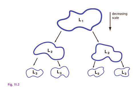
The passage of energy to smaller scales: eddies at large scale break up into ones at smaller scale, thereby transferring energy to smaller scales. The eddies in reality are embedded within each other. If the passage occurs between eddies of similar sizes (*i.e.*, if it is spectrally local), the transfer is said to be a cascade. This is Figure 11.2 from Vallis (AOFD).

We may first ask at what length scale does the viscosity become a dominant player. As useful tools we will recall dimensional analysis and the Reynolds number, which quantified the relative importance of inertial over viscous forces.

Re = \frac{UL}{\nu}

If we know that at the largest (think, geophysical) scales the viscosity is negligible (large $Re$ ), we could say that the viscosity becomes more important than turbulent motion at the scale at which $Re \approx 1$ . From there, we can define the viscous length scale as:

L_\nu = \frac{\nu}{U}

What are some characteristic values of $L_\nu$ in the ocean and in the atmosphere? An ocean flow with $U \approx 10^{-1}$ m/s and viscosity of $\nu \approx 10^{-6}$ m $^2$ /s gives $L_\nu \approx 10^{-5}$ m, or, one hundredth of a millimeter. In the atmosphere with $U \approx 10$ m/s and viscosity of $\nu \approx 10^{-5}$ m $^2$ /s, we get $L_\nu \approx 10^{-6}$ m, or, one micron. These are obviously very small scales.

Kolmogorov’s hypotheses and scales

To answer what happens to the flow statistics between the largest scales at which the turbulence is generated and the smallest scales at which viscosity dissipates all mechanical energy into heat, Kolmogorov (1941) proposed a new theory of turbulence based on three hypotheses. Kolmogorov’s three turbulence hypotheses are:

Hypothesis of local isotropy: At sufficiently high $Re$ and sufficiently small $L$ , the turbulence is locally isotropic, i.e. the flow statistics at a point are the same in all directions. In other words, the small-scale turbulence is homogeneous and has no preferred direction.
First similarity hypothesis: At sufficiently high $Re$ and sufficiently small $L$ , the flow statistics have a universal form that is uniquely determined by the viscosity $\nu$ and the energy dissipation rate $\varepsilon$ . In other words, small-scale turbulence is independent of the large-scale flow features such as the geometry and boundary conditions.
Second similarity hypothesis: At sufficiently high $Re$ and and sufficiently large $L$ , the flow statistics have a universal form that is uniquely determined by the energy dissipation rate $\varepsilon$ , and that is independent of viscosity $\nu$ . In other words, large-scale turbulence is governed by turbulent eddy dissipation and is independent of molecular viscosity.

The energy dissipation rate $\varepsilon$ comes straight from the TKE budget equation (8.42) and is defined as:

\varepsilon = \nu \overline{\nabla \mathbf{u}' \cdot \nabla \mathbf{u}'}

In a nutshell, Kolmogorov’s three hypotheses state that a turbulent flow at sufficiently small scales is the same looking in all directions, that statistically all such turbulent flows are the same, and that they are uniquely determined by either by energy dissipation rate alone, or by the energy dissipation rate and viscosity, depending on the scale. Through dimensional analysis, Kolmogorov also introduced three fundamental turbulent scales, now commonly known as Kolmogorov scales: The Kolmogorov length scale $\eta_k$ , the velocity scale $u_\eta$ , and the time scale $\tau_\eta$ .

Let’s use dimensional analysis to determine the length scale $\eta_k$ . Following Kolmogorov’s first similarity hypothesis, we assume that $\eta_k$ is a function of only $\nu$ and $\varepsilon$ :

\eta_k = f(\nu, \varepsilon) = \nu^a \varepsilon^b

The powers $a$ and $b$ can be determined by matching the dimensions on both sides:

L = \left( L^2 T^{-1} \right)^a \left( L^2 T^{-3} \right)^b

which leads to:

1 = 2a + 2b

0 = -a - 3b

so we arrive at $a = 3/4$ and $b = -1/4$ , giving us the Kolmogorov length scale:

\eta_k = \left( \frac{\nu^3}{\varepsilon} \right)^{1/4}

This is the scale at which the energy dissipation by molecular diffusion balances the energy input by the mean flow. (The subscript $k$ stands for “Kolmogorov”, and although it is not commonly used in the literature, here I use it to avoid a notion conflict with $\eta$ used for surface elevation.)

Following the same approach, we can derive the Kolmogorov time scale:

\tau_\eta = \left( \frac{\nu}{\varepsilon} \right)^{1/2}

which is the time scale at which the smallest coherent eddy can exist.

Finally, the Kolmogorov velocity scale is:

u_\eta = \left( \varepsilon \nu \right)^{1/4}

Any flow feature at scales smaller than these is governed by viscous dissipation of kinetic energy into heat.

Examining the Reynolds number using the Kolmogorov scales indeed shows that it reduces to unity, consistent with Eq. 8.45:

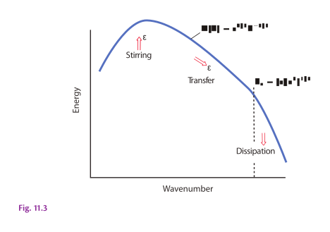
Re_\eta = \frac{u_\eta \eta}{\nu} = \frac{\left( \varepsilon \nu \right)^{1/4} \left( \nu^3/\varepsilon \right)^{1/4}}{\nu} = 1

Figure 8.3.
The energy spectrum in three-dimensional turbulence, in the theory of Kolmogorov (1941). Energy is supplied at some rate $\varepsilon$ ; it is cascaded to small scales, where it is ultimately dissipated by viscosity. There is no systematic energy transfer to scales larger than the forcing scale, so here the energy falls off. This is Figure 11.3 from Vallis (AOFD).

Now, we may ask, how is the turbulent energy distributed across the scales? Kolmogorov’s scales only tell us about the smallest scales of turbulence, at which its energy is dissipated by viscosity into heat. However, if his hypotheses are correct and the turbulence statistics are indeed universal across scales, we should be able to determine the distribution of turbulent energy across all scales by dimensional analysis. Define the energy spectrum $E(k)$ as the energy per unit mass per unit wavenumber:

E = \frac{1}{2} \int \mathbf{u}'^2(k)\ dk = \int E(k)\ dk

What is the form of the energy spectrum $E(k)$ ? Kolmogorov’s second similarity hypothesis states that the energy spectrum is universal and uniquely determined by the energy dissipation rate $\varepsilon$ . If that is true, then it must be some function of $\varepsilon$ and $k$ :

E(k) = F(\varepsilon, k)

The dimensions of $E(k)$ are $L^3 T^{-2}$ . Since the wavenumber $k$ has dimensions of $L^{-1}$ and thus no temporal dependence, the only way it can match the dimensions of $E(k)$ is if the energy spectrum scales with $\varepsilon^{2/3}$ (as this is the only scaling for $\varepsilon$ that will satisfy the time dimension of $E(k)$ ):

E(k) = \varepsilon^{2/3} G(k)

\frac{L^3}{T^2} \sim \frac{L^{4/3}}{T^2} G(k)

where $G(k)$ is some yet to be determined function of $k$ . Then, by dimensional analysis, $g(k)$ must have dimensions of $L^{5/3}$ , making the energy spectrum:

E(k) = \mathcal{K} \varepsilon^{2/3} k^{-5/3}

where $\mathcal{K}$ is a constant not determined by Kolmogorov’s theory. The functional form of $E(k)$ is known as the Kolmogorov 5/3 law and is illustrated in Figure 8.3.

Summary

In this chapter, we covered:

Reynolds decomposition of turbulent flows into mean and fluctuating components;
The turbulent energy spectrum and its distribution across scales;
Kolmogorov’s similarity hypotheses and dimensional analysis leading to the -5/3 law;
The turbulent energy cascade from large to small scales in 3D turbulence;
The role of energy dissipation rate $\varepsilon$ in determining the energy spectrum.