Chapter 9

Boundary layers

Boundary layers occur when a fluid flows over some kind of boundary, whether rigid or free, stationary or moving. They are both interesting and convenient because they constrain the flow near the boundary and thus allow simplifications that may lead to analytical solutions. They are important because they are often the dominant flow structure in geophysical flows. For example, a planetary boundary layer separates the atmosphere from the surface of the Earth. The surface beneath the planetary boundary layer may be rigid (land or sea ice) or free (ocean), and its roughness and thermodynamic properties may vary greatly from place to place. The most common geophysical boundary layers are the planetary boundary layer in the atmosphere (whether over land or water) and the upper-ocean mixed layer. Boundary layers also exist at the bottom of the ocean where the flow interacts with the seafloor, as well as where the air and water are directly impacted by surface waves. In this chapter, we start from the simplest boundary layer, a channel flow, and derive the stress and mean velocity profiles in laminar flows. Then, we zoom into the vertical structure of the boundary layer in turbulent flows, and examine different regimes that occur depending on the distance from the boundary.

Governing equations

A channel flow is a classic problem in fluid mechanics that is both relevant to engineering applications, and analogous to larger-scale geophysical flows. We begin by setting up the problem and establishing the governing equations and the notation that we will use. Then, we will explore some analytical and numerical solutions for the time-mean flow structure within the channel.

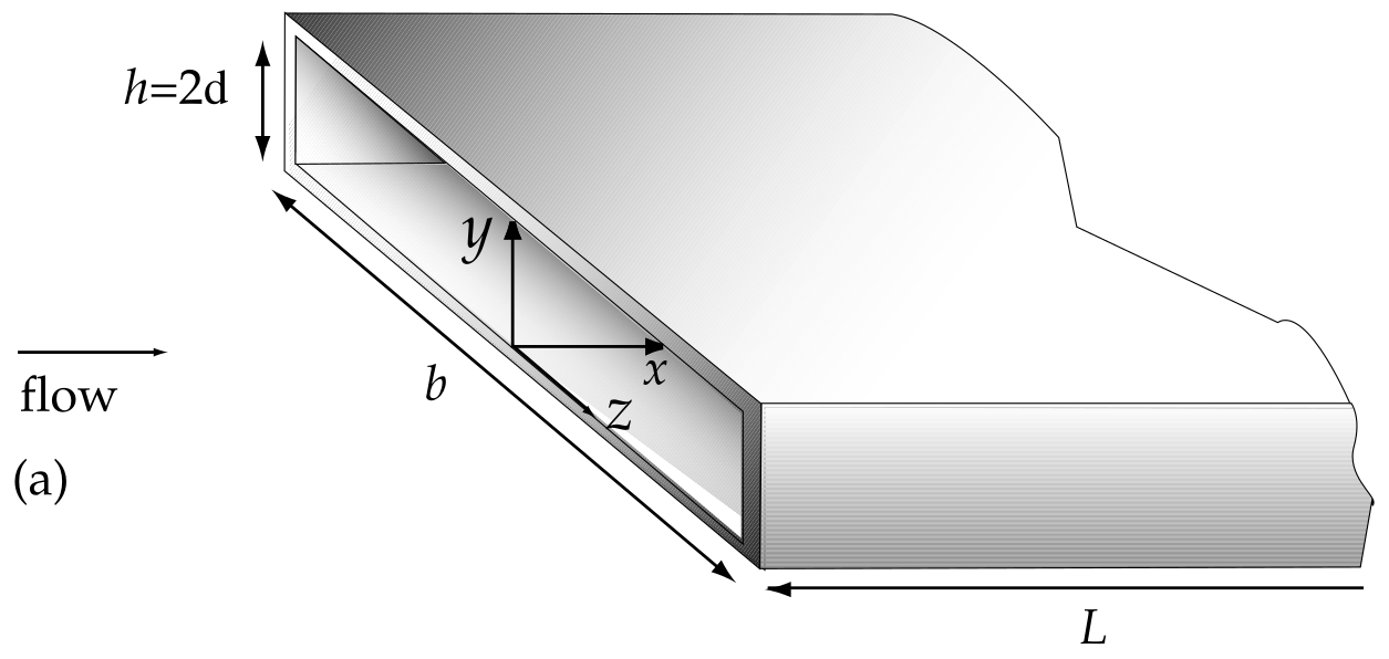
Sketch of a channel flow. The height of the channel is and the flow is in the direction. Although the vertical and the c — Figure 9.1.
Sketch of a channel flow. The height of the channel is $h$ and the flow is in the $x$ direction. Although the vertical and the cross-stream coordinates are denoted as $y$ and $z$ here, respectively, we will be using the opposite notation with $z$ being the vertical coordinate and $y$ the cross-stream coordinate. This is Figure 7.1a from Pope (2001).

Let’s examine a flow in a channel between two flat plates, spaced apart by a a distance $h = 2\delta$ , such that $\delta$ represents the centerline distance between the plates (Fig. 9.1). The channel is long ( $L \gg \delta$ ) and wide (width $\gg \delta$ ), so there is no variability in the $x$ and $y$ directions. The mean flow is predominantly in the $x$ direction, so if the velocity is defined as having components $u$ , $v$ , and $w$ in the streamwise, spanwise, and vertical directions, respectively, then:

\overline{u}(z) > 0

\overline{v} = 0

For simplicity, we won’t consider what happens at the very entrance into the channel where the flow develops, and we’ll only consider the fully developed flow well into the channel such that $\partial \overline{u}/\partial x = 0$ . Thus, from a statistical point of view, this is a stationary, one-dimensional flow that varies only in the $z$ direction.

As the simplest possible attempt to describe the turbulence in this scenario, let’s characterize the flow using a Reynolds number based on the bulk velocity:

Re \equiv \frac{\left<\overline{u}\right> 2 \delta}{\nu}

where $\left<\overline{u}\right>$ is the mean velocity in the channel (often also called bulk velocity):

\left< \overline{u}\right> = \frac{1}{\delta} \int_0^{\delta} \overline{u}(z)\ dz

Another useful Reynolds number is the one based on the centerline distance between the plates:

Re_0 \equiv \frac{u_0 \delta}{\nu}

where $u_0$ is the centerline velocity $u(z=\delta)$ . Based on laboratory experiments, we know that the channel flow is laminar for $Re < 1350$ and turbulent for $Re > 1800$ , with transitional effects observable up to $Re \approx 3000$ . Let’s now take note to distinguish these two Reynolds numbers as the bulk Reynolds number $Re$ (Eq. 9.3) and the centerline Reynolds number $Re_0$ (Eq. 9.5).

Next, let’s attempt to describe the vertical structure of the flow within the channel based on the governing equation for the mean velocity $\overline{u}(z)$ . Start from the Reynolds-averaged Navier-Stokes equation for $\overline{u}$ (Eq. 8.31):

\frac{\partial \overline{u}}{\partial t} + \frac{\partial \overline{u}\, \overline{u}}{\partial x} + \frac{\partial \overline{v}\, \overline{u}}{\partial y} + \frac{\partial \overline{w}\, \overline{u}}{\partial z} = - \frac{1}{\rho} \frac{\partial \overline{p}}{\partial x} + \nu \left( \frac{\partial^2 \overline{u}}{\partial x^2} + \frac{\partial^2 \overline{u}}{\partial y^2} + \frac{\partial^2 \overline{u}}{\partial z^2} \right) - \frac{\partial}{\partial x}\overline{u'u'} - \frac{\partial}{\partial y}\overline{u'v'} - \frac{\partial}{\partial z}\overline{u'w'}

For an incompressible flow, the continuity is $\nabla \cdot \overline{\mathbf{u}} = 0$ , which is effectively $\partial \overline{w}/\partial z = 0$ since the flow doesn’t vary in the $x$ and $y$ directions. $\overline{w}$ must be zero as we can’t have any flow through the walls of the channel, and so continuity requires that $\overline{w}$ is zero everywhere. Accounting for stationarity ( $\partial \overline{u}/\partial t = 0$ ), homogeneity in the $x$ and $y$ directions ( $\partial \overline{u}/\partial x = \partial \overline{u}/\partial y = 0$ ), and the fact that $\overline{w} = 0$ , Eq. 9.6 greatly simplifies to:

\frac{\partial \overline{p}}{\partial x} = \rho \nu \frac{\partial^2 \overline{u}}{\partial z^2} - \rho \frac{\partial}{\partial z}\overline{u'w'}

This stationary, one-dimensional flow is thus driven by the streamwise pressure gradient that is balanced by the normal viscous stress and the cross-stream Reynolds stress (that is, the vertical flux of horizontal momentum). The above can be further simplified to:

\frac{\partial \overline{p}}{\partial x} = \frac{\partial \tau}{\partial z}

where stress $\tau$ is the sum of the viscous and the turbulent Reynolds stresses:

\tau = \rho \left( \nu \frac{\partial \overline{u}}{\partial z} - \overline{u'w'} \right)

Since the mean flow is stationary (even though instantaenous flow is not!), the streamwise pressure gradient that drives it must be constant, and so does the vertical stress gradient as well:

\frac{\partial \tau}{\partial z} = \text{constant}

Assuming symmetry around the centerline of the channel requires that the stress there is zero, as there should not be any mean transport through the centerline. Integrating the above from $z=0$ to $z=\delta$ we get:

\tau(z) = a z + b

where $a$ and $b$ are constants. Use the boundary conditions $\tau(z=0) = \tau_w$ and $\tau(z=\delta) = 0$ to get:

\tau(z) = \tau_w \left( 1 - \frac{z}{\delta} \right)

where $\tau_w$ is the so-called wall stress whose value is yet to be determined. The stress thus decreases linearly from $\tau_w$ at the bottom wall to zero at the centerline, reaching $-\tau_w$ at the top wall.

As we do not yet have an expression for the the turbulent Reynolds stress in terms of any mean quantity, we cannot yet discuss the velocity profile in the general case. However, we can explore two limiting cases: laminar flow where the turbulent Reynolds stress is negligible, and turbulent flow where the turbulent Reynolds stress is dominant. If we can establish the velocity profiles in the two limiting cases, and the regions in the channel where each case is valid, we can then piece together a more complete picture of the flow structure within the channel.

Laminar flow

What does the velocity profile look like in the case of laminar flow? We can drop the Reynolds stress term in Eq. 9.9 and combine it with Eq. 9.12 to get:

\frac{\partial \overline{u}}{\partial z} = \frac{\tau_w}{\rho \nu} \left(1 - \frac{z}{\delta}\right)

Integrate the above with respect to $z$ to get:

\overline{u}(z) = \frac{\tau_w z}{\rho \nu} \left(1 - \frac{z}{2\delta} \right)

The velocity profile thus has a quadratic form that reaches zero at either wall (Fig. 9.2), and that has a centerline value of:

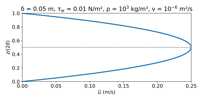
u_0 = \overline{u}(z=\delta) = \frac{\tau_w \delta}{2 \rho \nu}

Figure 9.2.

Mean velocity profile in laminar channel flow, for the flow parameters given in the title.

The preceding equations determine the stress and velocity profiles strictly in laminar flows, i.e. for relatively small Reynolds numbers. $\tau_w$ remains an unknown parameter, but it can be determined if the centerline velocity is known and if the flow in the entire channel is laminar.

Now, let’s see what the profiles may look like in turbulent flows.

Turbulent flow

Figure 9.3.

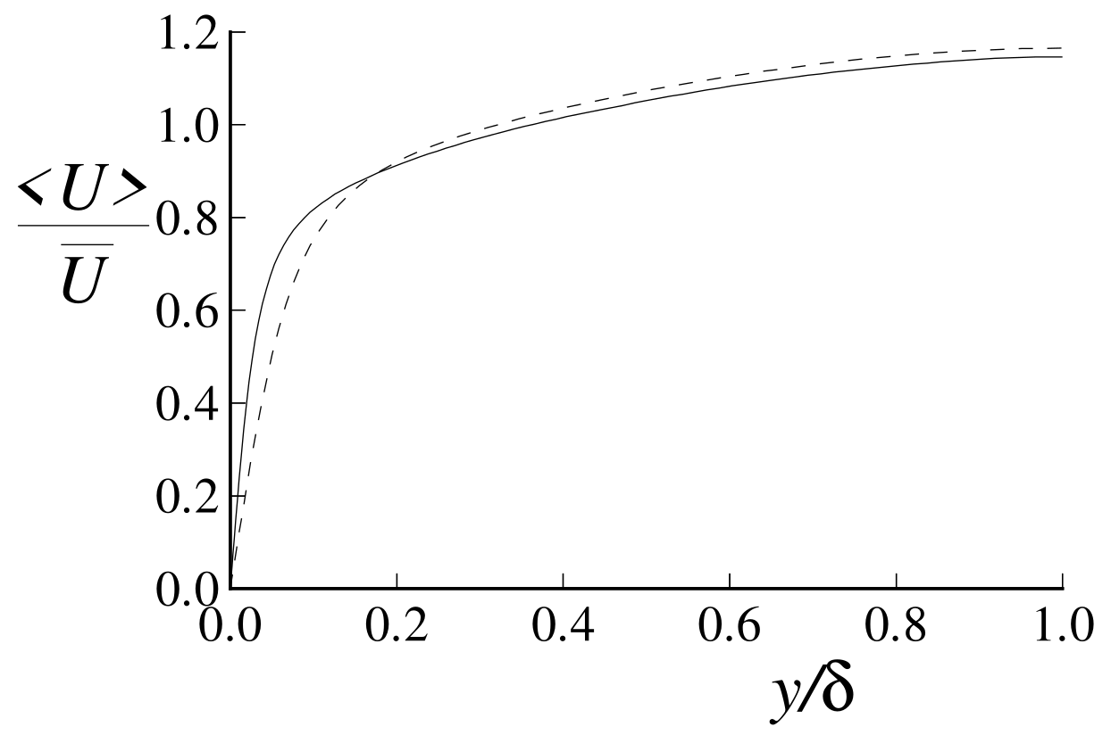
Mean velocity profile normalized by the bulk velocity in a fully developed turbulent channel flow, from the DNS of Kim et al. (1987). Dashed and solid lines are for $Re = 5,600$ and $Re = 13,750$ , respectively. Note that in the axis labels, $y$ is the vertical coordinate and the angle brackets and overline denote averaging in the opposite sense from our notation in the main text. This is Figure 7.2 from Pope (2001).

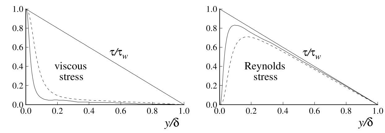
As in Fig. , but for the vertical profiles of the viscous and turbulent Reynolds stresses. This is Figure 7.3 from . — Figure 9.4.
As in Fig. 9.3, but for the vertical profiles of the viscous and turbulent Reynolds stresses. This is Figure 7.3 from Pope (2001).

In the laminar case, we were able to analytically derive the velocity and stress profiles. However, in the turbulent case, the problem is more complex and analytical solutions are not feasible due to the presence of the turbulent Reynolds stress term. Direct Numerical Simulations (DNS) reveal what a turbulent velocity profile in a channel may look like (Fig. 9.3).

At the boundaries, we can’t have any flow through the walls of the channel, the velocity and thus the turbulent Reynolds stresses must be zero, and so the wall shear stress must be entirely due to the viscosity:

\tau_w = \rho \nu \left( \frac{\partial \overline{u}}{\partial z} \right)_{z=0}

Recall from Eq. 9.9 that the stress $\tau$ is always composed of the viscous and turbulent parts. However, in turbulent flows, the relative contributions of the viscous and turbulent parts vary greatly as we move away from the wall. Fig. 9.3 shows how, in a well developed turbulent flow, the mean velocity increases as we move further away from the wall. At about 0.4 of the way toward the centerline, the time-mean velocity approximately equals the bulk velocity, and exceeds it as we approach the centerline. The profiles are also somewhat different depending on the Reynolds number, with the velocity profile being gentler for a smaller Reynolds number flow. This is somewhat intuitive, as we know that the turbulent Reynolds stresses are much more effective at mixing than the molecular viscosity. A somewhat less turbulent flow is thus expected to have a gentler velocity, as its momentum is being mixed more by viscosity and less by turbulence.

What is the vertical structure of the viscous and turbulent Reynolds stresses then? We don’t have an analytical solution for the stress profiles, like we did in the laminar case, but we can look at the DNS data to see what the profiles look like. Fig. 9.4 shows the vertical profiles of the viscous and turbulent Reynolds stresses based on the DNS data of Kim et al. (1987). Consistent with Eq. (9.12), the total stress decreases linearly from $\tau_w$ at the wall to zero at the centerline. However, the stress components vary differently between one another. The viscous stress makes up all of the stress at the very wall, and rapidly decreases as we move away from the wall. The turbulent stress, on the other hand, is zero at the wall, and rapidly increases as we move away from the wall. At a lower Reynolds number, the turbulent stress reaches a lower peak value, with the peak being further away from the wall, compared to the higher Reynolds number case.

It is clear from Figs. 9.3 and 9.4 that viscosity (via the Reynolds number) and the wall stress $\tau_w$ are important parameters for the vertical structure of the flow. These quantities, alongside the fluid density $\rho$ , allow us to define the viscous scales (length and velocity) that govern the the flow near the wall. These are the friction velocity:

u_* \equiv \sqrt{\tau_w/\rho}

and the viscous length scale:

\delta_\nu \equiv \nu/u_*

The viscous length scale, also known as the wall unit, quantifies the distance from the wall at which the smallest turbulent motions are felt, and within which all dissipation of kinetic energy is done by viscosity. On the other hand, the friction velocity $u_*$ is not a physical velocity of the flow at any single location, but rather a scaling parameter with the units of velocity that characterizes the flow near the wall. Mathematically, you can think of it as the wall shear stress expressed in units of velocity.

It’s useful to also distinguish between the viscous Reynolds number:

Re_\nu \equiv \frac{u_* \delta_\nu}{\nu}

which, as we saw before, is identically unity, and the friction Reynolds number, defined as:

Re_\tau \equiv \frac{u_* \delta}{\nu}

Figure 9.5.
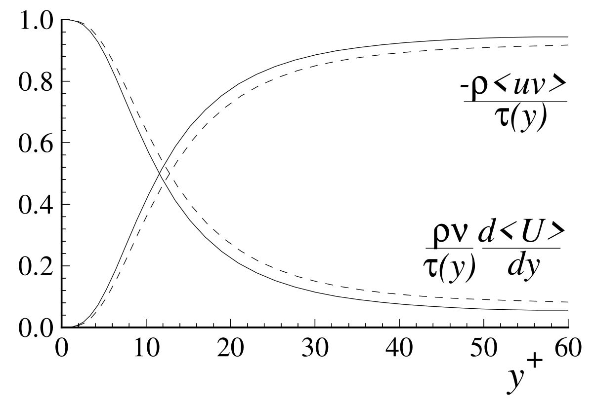
Profiles of the fractional contributions of the viscous and turbulent Reynolds stresses to the total stress, based on the DNS data of Kim et al. (1987), as in Figs. 9.3 and 9.4. This is Figure 7.4 from Pope (2001).

Based on the viscous length scale, we define a new non-dimensional coordinate $z^+$ as:

z^+ \equiv \frac{z}{\delta_\nu} = \frac{u_* z}{\nu}

which is the physical vertical distance normalized by the viscous length scale. This quantity thus allows us to see how the flow properties vary with the distance expressed as a number of wall units. One example of that is the fractional contribution of the viscous and turbulent stresses to the total stress, shown in Fig. 9.5. The fact that the stress contribution profiles between the lower and higher Reynolds number cases almost collapse on one another when plotted against $z^+$ (compare with the two cases in Fig. 9.4) provides a hint into the usefulness of this non-dimensionalization. It demonstrates the universality of the turbulent flow structure, and allows us to make some general statements about the flow structure that are independent of the Reynolds number. This figure shows that the viscous and turbulent stresses become approximately equal at about $z^+ \approx 12$ . Some useful criteria for $z^+$ in characterizing the flow regimes are:

z^+ \lesssim 5 \quad \text{(viscous sublayer)}

5 \lesssim z^+ \lesssim 50 \quad \text{(viscous wall region)}

z^+ \gtrsim 50 \quad \text{(outer region)}

As a rule of thumb, we claim that the viscous sublayer is predominantly laminar, governed by viscosity, and does not permit turbulent eddies; the outer region is dominated by turbulence and the viscous stress is relatively negligible; finally, the viscous wall region is a transition zone between the two, with both viscous and turbulent stresses being important.

Let’s now examine in more detail each of these regions and see if flow structure varies significantly between them.

Velocity structure in various wall regions

Now, let’s look at the time-mean velocity profiles in the turbulent channel flow, and in various regions near and away from the wall. When fully developed, such flow is completely determined by the fluid density $\rho$ , the kinematic viscosity $\nu$ , the channel half-height $\delta$ , and the friction velocity $u_*$ , because:

u_* = \sqrt{- \frac{\delta}{\rho} \frac{\partial \overline{p}}{\partial x}}

Between these parameters, there are only two independent non-dimensional groups that can be formed: $z/\delta$ and $Re_\tau = u_* \delta / \nu$ . It should then be possible to express the velocity profile as a function of these parameters:

\overline{u}(z) = u_* F\left(\frac{z}{\delta}, Re_\tau\right)

where $F$ is some yet-to-be-determined non-dimensional function. However, since both the viscous stress and the turbulent production are determined by the mean shear $\partial \overline{u}/\partial z$ , it may be more useful to seek the form of the velocity profile in terms of the mean shear:

\frac{\partial \overline{u}}{\partial z} = \frac{u_*}{z} \Phi\left(\frac{z}{\delta}, \frac{z}{\delta_\nu}\right)

where $\Phi$ is, like $F$ before, some yet-to-be-determined non-dimensional function, and the proportionality to $u_*/z$ is proposed on dimensional grounds. Notice that the second argument of $\Phi$ , $z/\delta_\nu$ (which we also defined earlier as $z^+$ ), is equivalent to $Re_\tau z/\delta$ , so it is useful to see $\Phi$ as a function of two non-dimensional heights, one characteristic of the boundary layer and another of the viscous sublayer. The nondimensional heights $z/\delta$ and $z/\delta_\nu$ thus capture all relevant flow parameters, namely $\rho$ , $\nu$ , $\delta$ , $\tau_w$ , as well as the distance from the wall $z$ .

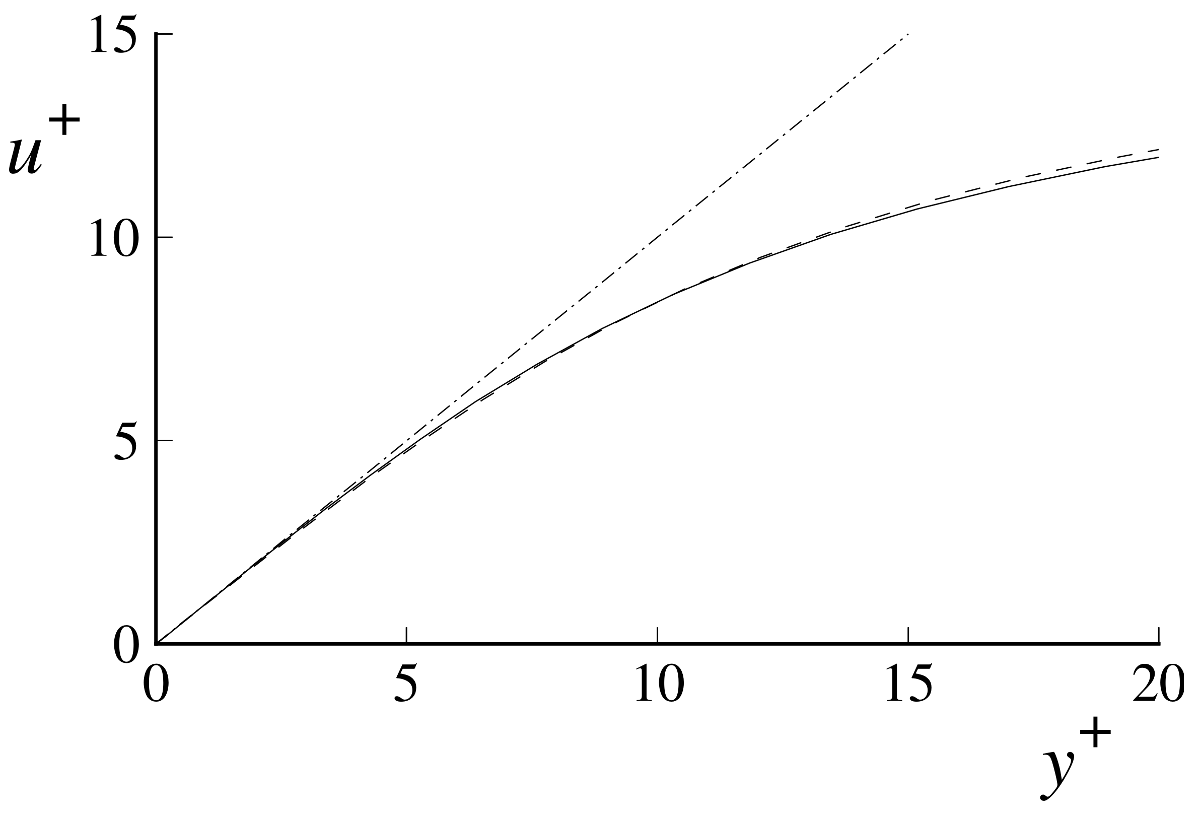
Near-wall profiles of mean velocity from the DNS data of Kim et al. (1987): dashed line, ; solid line, ; dot-dashed line — Figure 9.6.
Near-wall profiles of mean velocity from the DNS data of Kim et al. (1987): dashed line, $Re = 5,600$ ; solid line, $Re = 13,750$ ; dot-dashed line, $u^+ = z^+$ . This is Figure 7.5 from Pope (2001).

Let’s focus for now on the region closest to the wall, which may include the viscous sublayer and extend somewhat beyond it. Prandtl (1925) hypothesized that at high Reynolds numbers, there is a region very near the wall ( $z \ll \delta$ ), called the inner layer, in which the mean velocity profile is entirely governed by viscosity, and is independent of the boundary layer size $\delta$ and the centerline velocity $u_0$ . Thus, as $z/\delta \to 0$ , $\Phi(z/\delta, z/\delta_\nu) \to \Phi_I(z/\delta_\nu)$ , so in this region Eq. (9.27) reduces to:

\frac{\partial \overline{u}}{\partial z} = \frac{u_*}{z} \Phi_I\left(\frac{z}{\delta_\nu}\right) = \frac{u_*}{z} \Phi_I\left(z^+\right)

Since $\Phi_I$ is a function of $z^+$ and it’s the function that we want to determine, let’s express the other variables in Eq. (9.28) in terms of $z^+$ as well. To do that, we introduce the non-dimensional velocity which is the velocity normalized by the friction velocity:

u^+ \equiv \frac{\overline{u}}{u_*}

Recalling that $u_* = \nu/\delta_\nu$ and that $z^+ = z/\delta_\nu$ , we can express Eq. (9.28) as:

\frac{\partial u^+}{\partial z^+} = \frac{1}{z^+} \Phi_I\left(z^+\right)

The non-dimensional velocity $u^+$ is thus a function of $z^+$ alone:

u^+ = f_w(z^+)

where $f_w$ is the wall function, expressed in terms of $z^+$ as:

f_w(z^+) = \int_0^{z^+} \Phi_I(z) dz

Equations (9.31)-(9.32) make the so-called law of the wall. There is copious experimental and DNS evidence that $f_w(z^+)$ is a universal function for boundary layers in general. Let’s find the form of this function for small and large values of $z^+$ .

In the viscous sublayer, we can establish from Eq. (9.16) and the no slip boundary condition that:

f_w(0) = 0

f'_w(0) = 1

which implies that for very small values of $z^+$ , the wall function is:

f_w(z^+) \approx z^+

The validity of the linear scaling of the velocity with $z^+$ in the inner layer is shown based on DNS data in Fig. 9.6. Up to about $z^+ \approx 5$ , the velocity scales linearly with $z^+$ , as expected from the viscous sublayer. However, beyond $z^+ \approx 5$ , the velocity scales differently and we need to seek a different functional form for $f_w(z^+)$ . Based on the data, it seems like the function may have a logarithmic dependence on $z^+$ .

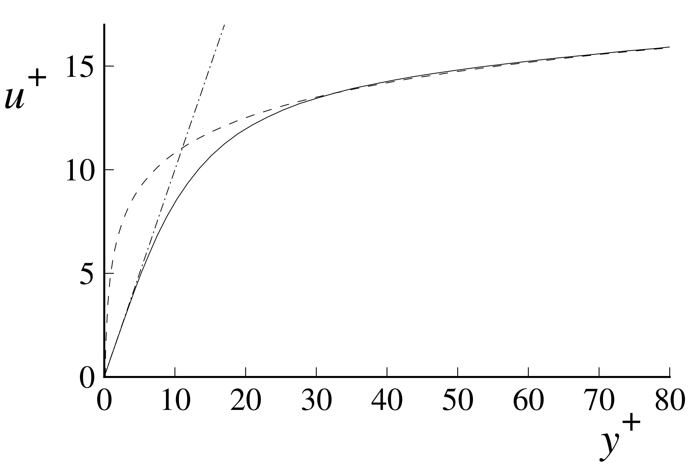
Near-wall profiles of mean velocity: Solid line, DNS data of , ; dot-dashed line, ; dashed line, the log-law. This is Fi — Figure 9.7.
Near-wall profiles of mean velocity: Solid line, DNS data of Kim et al. (1987), $Re = 13,750$ ; dot-dashed line, $u^+ = z^+$ ; dashed line, the log-law. This is Figure 7.6 from Pope (2001).

Away from the wall, we can suppose that the viscosity plays smaller role, and thus $\Phi_I(z^+)$ reduces to a constant, experimentally determined to be $1/\kappa$ , where $\kappa$ is the von Kármán constant and approximately equal to $0.41$ :

\Phi_I(z^+) = \frac{1}{\kappa}, \quad \text{for } \frac{z}{\delta} \ll 50 \text{ and } z^+ \gg 1

In this region, the velocity shear is then:

\frac{\partial u^+}{\partial z^+} = \frac{1}{\kappa z^+}

which integrates to:

u^+ = \frac{1}{\kappa} \ln(z^+) + C

where $C$ is an integration constant, experimentally determined to be about $5.2$ . Returning back to our dimensional variables, we can express the velocity profile as:

\overline{u}(z) = u_* \left[ \frac{1}{\kappa} \ln\left(\frac{z}{\delta_\nu}\right) + 5.2 \right]

The log-law is demonstrated based on DNS data in Fig. 9.7, and its universality (i.e. independence of the Reynolds number) is demonstrated based on experimental data in Fig. 9.8.

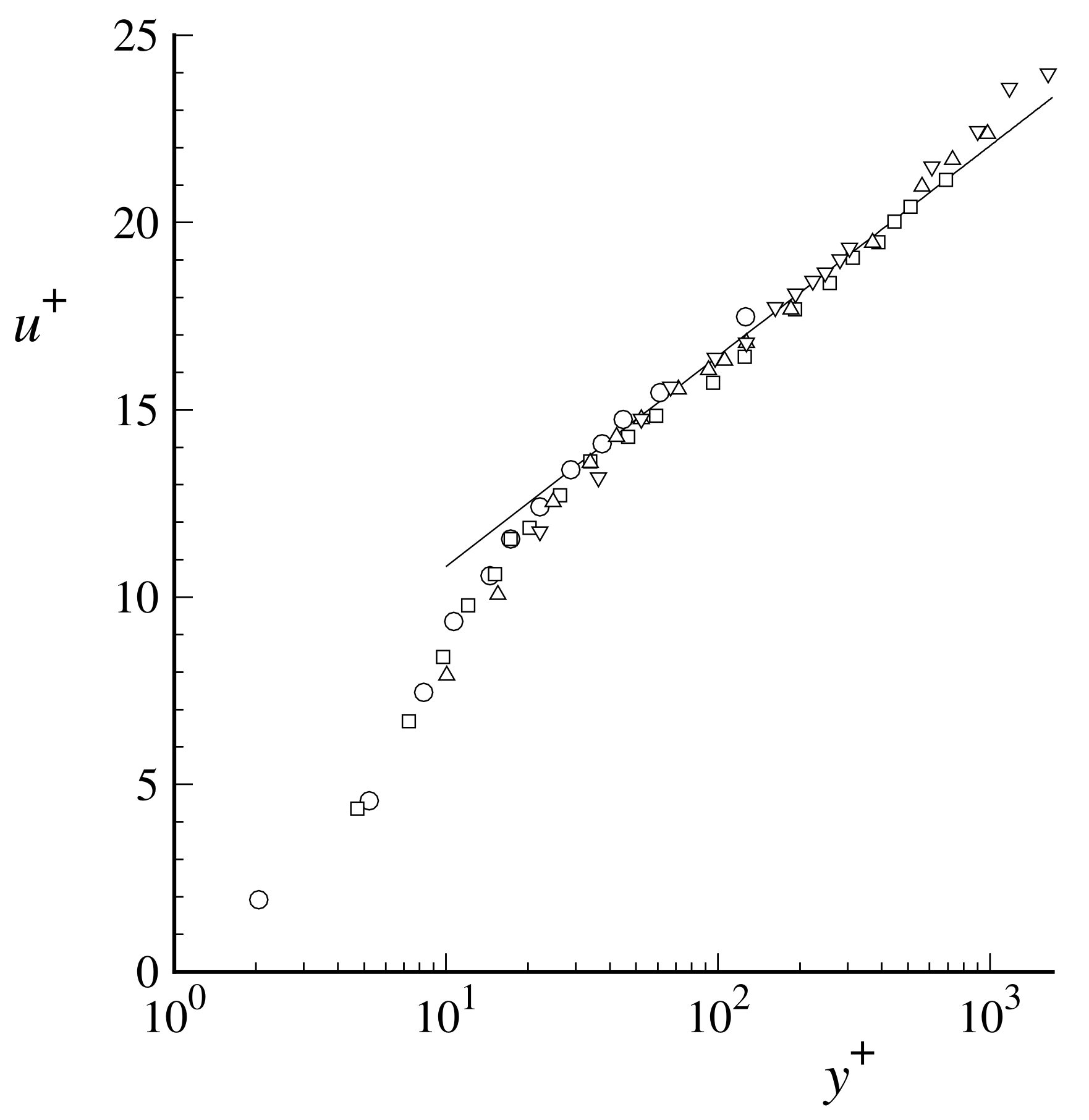
Mean velocity profiles in fully developed turbulent channel flow measured by : Circles, ; squares, ; upward triangles, ; — Figure 9.8.
Mean velocity profiles in fully developed turbulent channel flow measured by Wei and Willmarth (1989): Circles, $Re_0 = 2,970$ ; squares, $Re_0 = 14,914$ ; upward triangles, $Re_0 = 22,776$ ; downward triangles, $Re_0 = 39,582$ ; line, the log-law. This is Figure 7.7 from Pope (2001).

In summary, the velocity structure in the near-wall region of a turbulent boundary layer can be summarized as:

For $z^+ \lesssim 5$ (viscous sublayer), $u^+$ scales linearly with $z^+$ and likewise for $u$ scaling with $z$ ;
For $z^+ \gtrsim 50$ (log-law region), $u^+$ scales logarithmically with $z^+$ and likewise for $u$ scaling with $z$ ;
For $5 \lesssim z^+ \lesssim 50$ (viscous wall region), the velocity profile transitions between the two regimes above.

Exercises

Find the expression for the bulk velocity (see Eq. 9.4) of a laminar channel flow. How large is it compared to the centerline velocity $u_0$ ? How about the bulk Reynolds number relative to the centerline Reynolds number $Re_0$ ?
Consider a fully developed turbulent channel flow. The fluid viscosity is $\nu = 10^{-6}$ m $^2$ /s, the channel half-height is $\delta = 0.1$ m, and the friction velocity is $u_* = 0.1$ m/s. Assuming that the inner layer is negligible compared to the channel height and that the log-law applies throughout the channel, find the mean centerline velocity ( $\overline{u}$ at $z=\delta$ ) and the bulk velocity (Eq. 9.4).

Summary

In this chapter, we covered:

The structure of turbulent boundary layers and channel flows;
The law of the wall and its different regimes (viscous sublayer, buffer layer, log-law region);
Non-dimensional velocity and length scales based on the friction velocity $u_*$ ;
The universality of the log-law across different Reynolds numbers;
The relationship between mean velocity profiles and wall stress through the friction coefficient $C_f$ ;
Experimental validation of boundary layer theory using DNS and laboratory measurements.