Chapter 10
Surface gravity waves
In the previous chapter, we examined the structure of laminar and turbulent boundary layers over a rigid, stationary, flat wall. However, when the wind blows over the ocean surface, it generates waves that make the ocean surface irregular and moving. In this chapter, we study this “soft” and moving boundary between the atmosphere and the ocean, that is, the wavy ocean surface. The key restoring force for the surface waves, as we will soon see, is gravity, and so these waves are often called gravity waves, much like the waves we explored as a solution of the shallow water equations in Chapter Shallow water systems. In the first part of this chapter, we derive the solution for the small-amplitude (often called linear) waves, which is valid when the wave amplitude is much smaller than the wavelength and the water depth. This assumption allows for a relatively straightforward solution of the flow anywhere below the free wavy surface. Although simplistic in its approximations, the linear wave theory has been surprisingly successful in predicting the behavior of the waves even when the assumptions behind it are clearly violated. The linear wave theory remains the basis of modern wave prediction models that are used in operational weather and ocean forecasting. After deriving the linear wave solutions, we will explore their properties and derive some second-order quantities with implication for mean ocean circulation.
Small-amplitude wave derivation
Waves on the surface of a liquid have, within certain limits, an exact solution for which many useful properties can be derived. Modern ocean wave prediction models (Group, 1988; Tolman, 1991; Booij et al., 1999; Donelan et al., 2012) are based on this solution.
Governing equations
Key assumptions are that the fluid is incompressible (), inviscid (), and irrotational (). The inviscid assumption is required for the fluid to remain irrotational, and the irrotational property allows expressing the velocity field in terms of a scalar potential. Incompressibility implies that this theory works well for liquids (such as water on Earth or ancient Mars or liquid methane on Titan) but not for gases.
In irrotational flows, velocity has a scalar potential such that:
Incompressibility then dictates that:
This is called the Laplace equation, and it holds throughout the fluid. In two dimensions, horizontal and vertical, Eq. 10.2 is:
which is sufficient if we consider surface waves that propagate in the -direction and that are otherwise uniform in the -direction.
Although is allowed to vary in both space and time, the Laplace equation states that at any given time, anywhere in the interior of the fluid is determined by its values at the boundary (i.e. the boundary conditions). It does not, however, determine how evolves in time. One important property of the velocity potential is that it is not unique, i.e. there are infinitely many functions that satisfy the Laplace equation. For example, if is a velocity potential, then so is , where is a scalar constant, and so is , where is an arbitrary function of time. Another one is that a sum of any number of velocity potentials is also a velocity potential.
Now, to determine the time dependence of , we integrate the Euler equations of motion (introduced back in Conservation of momentum, see Eq. 4.29) to obtain a steady-state relationship between the pressure and the velocity of the fluid. The Euler equations in - plane are:
Now, recall that we require the flow to be irrotational, so:
which leads to:
We can use this to rewrite Eqs. 10.4-10.5 as:
Now, express the velocity components in the time derivatives as gradients of the velocity potential:
Integrating these equations with respect to and respectively, we obtain:
where and are integration constants that can vary in dimensions other than their respective dimension of integration. Since these equations have the same left-hand sides, their right-hand sides must be equal:
thus can only depend on time, and we get our final equation form called the Bernoulli equation:
The Bernoulli equation will serve as a dynamic free surface boundary condition as we proceed to derive the solutions for the surface gravity waves. At this time, notice also that the second and third term represent the kinetic and potential energy, respectively. This implies that the rate of change of the local value of the velocity potential will be governed by the sum of the kinetic energy, potential energy, and pressure energy per unit mass of the fluid.
Boundary conditions
Now that we established the governing equations to solve, we need to specify the boundary conditions to determine the velocity potential in the interior. We will rely on a total of four boundary conditions:
-
Kinematic free surface boundary condition: This boundary condition determines the vertical velocity at the free surface by exploiting the fact that the Lagrangian (material) change of the vertical position is the vertical velocity itself:
Expressed in terms of the velocity potential, this boundary condition becomes:
-
Dynamic free surface boundary condition: We leverage the Bernoulli equation Eq. 10.15 at the free surface () and set the surface pressure to be zero:
-
Bottom boundary condition: The bottom is rigid and impermeable, so the vertical velocity is zero at the bottom:
where is the mean depth of the fluid.
-
Lateral boundary condition: At the lateral boundaries, since we’re seeking a wave solution, we know that the velocity potential must be periodic in the horizontal space as well as time:
where is the wavelength and is the period.
With these four boundary conditions, we are now equipped to solve for the velocity potential in the interior of the fluid.
Solution
Our key equation to solve is the Laplace equation (Eq. 10.2) for the velocity potential that varies in the horizontal and vertical direction and respectively, as well as time :
To solve this equation, we will rely on the method of separation of variables, where we assume that the solution can be written as a product of functions that depend on each coordinate separately:
We can start from the time-dependent part and recall the lateral boundary condition which states that the velocity potential must be periodic in time, which is true for sines and cosines (and any linear combination of them). For a sine function of a phase , this is true:
And expressing it as a function of time:
where is the angular frequency in units of radians per second, so that the phase has angle units (radians). Notice that we could have picked (and soon, we will) a cosine function instead of a sine function, and the solution would still be valid. With the choice of a sine for the time-dependent part of the potential, we write the full velocity potential as:
Insert this into Eq. 10.22 to get:
Divide by to get:
Can we separate this even further? Recall that and are functions of and respectively. If, for example, we hold constant and consider variations in , the first term would remain constant but the second term would not! You can arrive to the same conclusion by holding constant and varying . This would clearly violate Eq. 10.28, and so the only way that equation can hold is if both and are equal to the same constant but with opposite signs:
where is the separation constant. These can also be written as:
For real values of , the solutions to these equations are:
where , , , and are constants that are yet to be determined. We now write our intermediate solution for the velocity potential as:
Next, let’s attempt to constrain the -dependent part of the potential, . Recall the bottom boundary condition which for a flat bottom requires at . Then:
which implies . Insert this back into Eq. 10.34 to get:
Inserting this back into Eq. 10.35 we get:
Now, how about the free surface boundary condition? Recall the Bernoulli equation at with :
Denoting this equation as BE, we can evaluate it at the free surface using the Taylor expansion around :
To greatly simplify the algebra, this is where we invoke the small-amplitude approximation, which effectively states that if , then , , , and so on. This is where the linearization of the wave solution occurs, and it’s where it is possible to find wave solutions to a higher-order, such as those of the Stokes wave theory. For brevity, we keep only the first-order terms being the largest and write:
and from here we have the expression for the free surface elevation as function of the potential and time:
As by definition is a periodic displacement around the mean water level, its spatial and temporal average is zero, so must be zero as well, assuming that the surface pressure is negligible and is dropped from the Bernoulli equation. The surface elevation is then:
and so the constant must be such that the wave amplitude is:
and the constant is:
Insert this back to our intermediate solution for the velocity potential Eq. 10.38 and moving the minus sign into the -dependent part of the potential, we get:
which is our new intermediate solution for .
Let’s revisit again the lateral boundary conditions and recognize that , and are all valid solutions to the Laplace equation, which means that any combination of them is a valid wave solution. Same is true for where we chose a sine form, but we could have chosen a cosine form instead, or some combination of the two. This property of the velocity potential allows us to describe both standing and progressive waves with the same functional form for . Specifically:
is a valid velocity potential that belongs to a standing wave with amplitude . Recognizing that both the sines and cosines are valid forms for the - and -dependent parts of the velocity potential, and we can thus linearly combine them to obtain a valid velocity potential that belongs to a progressive wave, specifically:
A valid velocity potential that belongs to a progressive wave with amplitude is then:
The elevation that corresponds to this velocity potential is:
Equations (10.49) and (10.50) fully describe the spatial and temporal evolution of a wave with amplitude and wavenumber over mean water depth . The wave potential field for a linear, progressive gravity wave with m and rad/m, and its corresponding elevation, are shown in Fig. 10.1. The velocity potential for this wave has a positive maximum at the surface on the front face of the wave and a negative minimum at the surface on the back face of the wave. The potential is largest at the surface and decays exponentially with depth.
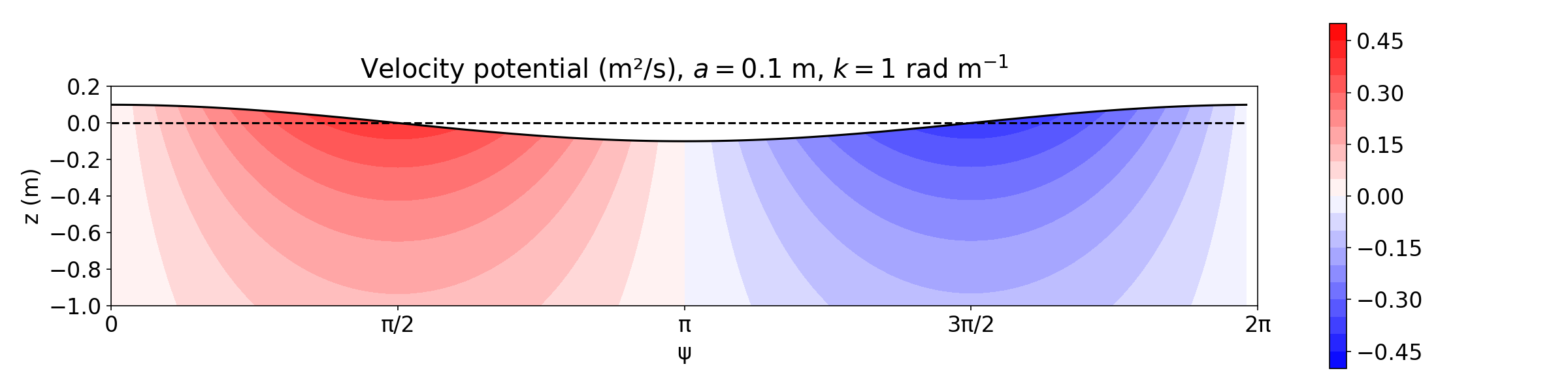
Wave elevation (black line) and velocity potential (color) for a linear wave with amplitude m and wavenumber rad m, in deep water ( m). The mean water level () is indicated by the horizontal dashed line. The wave is propagating from left to right.
In the deep water limit, the wave potential can be written more concisely as:
As we explore the wave kinematics, we will leverage this form for brevity.
Dispersion of gravity waves
An important property of surface gravity waves is that they disperse, meaning that waves of different frequencies (or wavenumbers) travel at different speeds. A dispersion relationship describes how the wavenumber changes as function of frequency. To derive it, we leverage the kinematic free surface boundary condition (Eq. 10.16), where, to the first order (recall our small-amplitude approximation), we have:
which leads to:
Simplifying on both sides, we arrive to:
which is the dispersion relationship for surface gravity waves. Wavenumber as function of frequency is shown in Fig. 10.2.
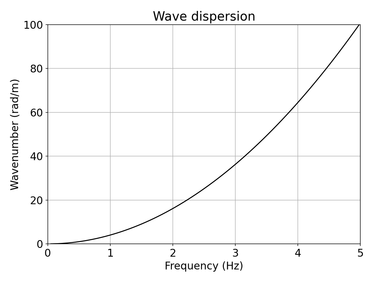
Wavenumber as function of frequency for the surface gravity waves in deep ( m) water. The wavenumber range is from to rad/m. The corresponding frequency range is from approximately to Hz.
Let’s now evaluate this dispersion relationship in the limits of shallow and deep water. In deep water, and so . Then:
So, in deep water, the frequency is not dependend on water depth, which we expected–the rigid bottom is so far away from the free surface that the waves don’t feel it at all. The frequency is dependent on the wavenumber and gravity only. In contrast, in shallow water, and so . Then:
or:
Here, the frequency depends on both the wavenumber and the water depth. So, as waves enter progressively shallower water, their frequency decreases. However, unlike in deep water where the frequency is nonlinearly dependent on wavenumber, in shallow water they are linearly correlated by .
An important wave property that directly follows from the dispersion relationship is that for the wave celerity, or phase speed, which is the speed at which the wave potential field and elevation propagate in the horizontal direction:
Like the dispersion relationship itself, the expression for the phase speed simplifies as well in the limits of shallow and deep water. In deep water, , and in shallow water, . It is no coincidence that this is the same expression that we found for the phase speed of Poincaré waves in the limit of negligible planetary rotation (Eq. 7.38).
Before we close this section, let’s remark on the fact that the dispersion relation for waves in water of arbitrary depth (Eq. 10.54) is nonlinear and transcendental in because of the hyperbolic tangent term. This means that although evaluating the frequency given the wavenumber is straightforward, the inverse problem of finding the wavenumber given the frequency is not trivial and requires a numerical approximation or iteration. Of course, both the deep and shallow water limits provide simple analytical expressions for as function of , but these are only valid in their respective limits.
Wave kinematics
With the velocity potential well defined in Eq. 10.51, the instantaneous wave-induced velocities can be readily obtained as:
The wave-induced velocity thus have the following properties:
-
It oscillates sinusoidally in both space and time, just like the wave elevation.
-
The horizontal and vertical velocities are exactly out of phase in both space and time.
-
Their magnitude scales with the wave amplitude and frequency, and decays exponentially with depth, their decay scale being proportional to .
The horizontal velocity is in phase with the wave elevation, which means that it reaches its maximum at the wave crest and minimum (maximum but in the opposite direction) at the wave trough. The vertical velocity is correspondingly positive and largest on the front face of the wave (where the elevation is increasing with time) and negative and largest in magnitude on the back face of the wave (where the elevation is decreasing with time). As an example, these velocities for a linear wave with amplitude m and wavenumber rad m, in deep water ( m), are shown in Fig. 10.3.
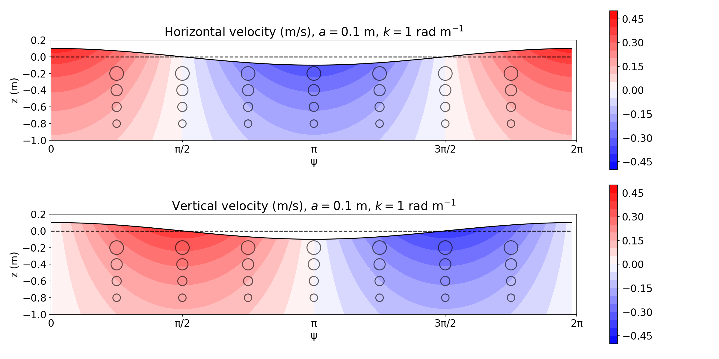
Wave elevation (black line) and horizontal (top) and vertical (bottom) velocities (color) for a linear wave with amplitude m and wavenumber rad m, in deep water ( m). Thin lines indicate the water particle trajectories.
Now that we have the velocities, it is instructive to look at how the water particles move in the wave field. The horizontal and vertical displacements can be obtained by integrating their respective velocities over time:
The displacements are thus closed orbits when evaluated at any fixed depth .
The wave-induced accelerations are also relevant because they govern the wave-induced forces on submerged bodies. They are simply a time derivative of the respective velocities:
Accelerations are a common measurement of ocean surface waves, especially on freely drifting platforms.
Mean Lagrangian velocity
It’s clear that averaging the instantaneous orbital velocities at any given fixed depth over one or more period yields zero. However, if we follow the water particles in Lagrangian sense, their average horizontal velocity will be non-zero because the particles move forward a larger distance than backward over the course of one period. This mean Lagrangian velocity is called the Stokes drift. We can find the expression for this mean residual drift by first recognizing that we can approximate the velocity at a particle position to the first order as:
The Stokes drift can then be obtained by averaging this material velocity over one period:
It can be easily shown by following the same procedure for the vertical velocity that the vertical Stokes drift is zero.
Relative to the instantaneous orbital velocity, the Stokes drift has an addition factor of (wave steepness), and it decays with depth twice as fast as the orbital velocity. This means that the Stokes drift induced by short waves is also confined to the near surface, whereas only longer waves such as swell can induce significant Stokes drift at the depth of several meters or more.
Although the Stokes drift has dimensions of velocity, it is not a true velocity at any given instant in time, but rather a mean Lagrangian drift of water particles. It thus cannot be directly measured with an Eulerian current meter, but instead can be inferred by tracking the trajectories of drifting buoys or surface floats. Fig. 10.4, from Curcic et al. (2016), shows trajectories of a five member cluster of surface drifters deployed during the GLAD experiment in the Gulf of Mexico in August 2012, in the aftermath of Hurricane Isaac. The observed drifter trajectories (black) are compared with simulated trajectories using only the Eulerian ocean current (green) and using the ocean current plus the Stokes drift (red). The inclusion of the Stokes drift significantly improves the agreement between the observed and simulated drifter trajectories, especially in the strongly forced region on the right side of the hurricane track. Although not exactly a measurement of the Stokes drift itself, it illustrates in a qualitative sense that the wave-induced Lagrangian drift contributed significantly to the final observed displacement of the drifters. This was also the first documented inference of Stokes drift in hurricane conditions.
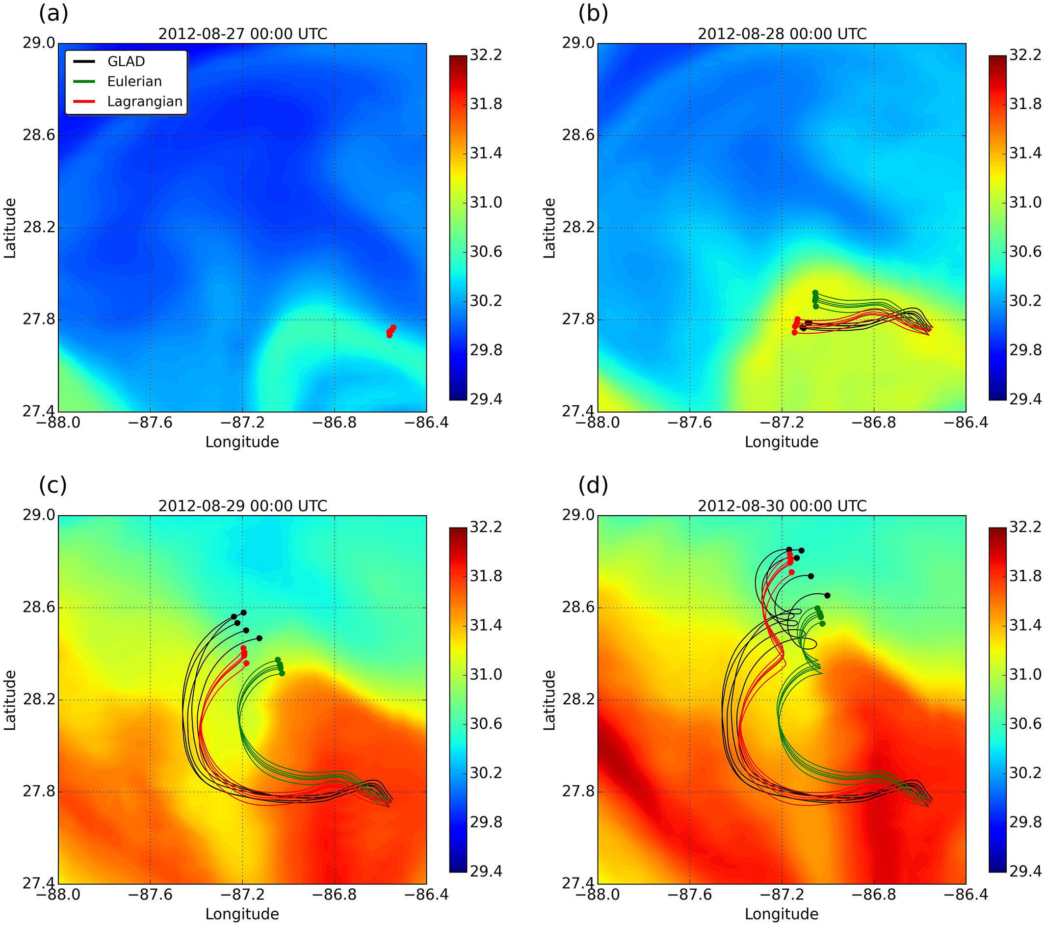
Trajectories of a five member cluster located in a strongly forced region on the right side of Hurricane Isaac track from 0000 UTC 27 to 30 August 2012. Observed (black) and simulated trajectories using the Eulerian (green; ocean current without Stokes drift) and Lagrangian (red; ocean current with Stokes drift) velocities started at the same initial positions as the GLAD drifters. The dots mark drifter locations valid on the time indicated on top of each panel. The color background shows simulated surface seawater density minus . Adapted from Curcic et al. (2016).
Wave groups
Waves of a given wavenumber and frequency are rarely alone and in reality the ocean surface is densely populated by a spectrum of waves with different wavenumbers and frequencies. The simplest case of this is if we considered two waves and their resulting elevation:
Superposing two waves with different wavenumbers leads to the formation of wave groups (Fig. 10.5).
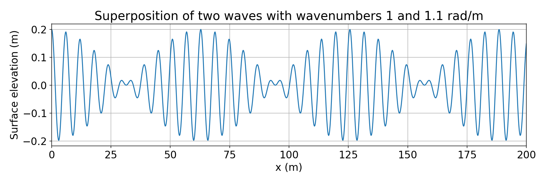
Superposition of two waves with wavenumbers 1 and 1.1 rad/m and amplitudes of 0.1 m.
Now, to see at what speed does the wave group propagate, write the wavenumbers and frequencies of independent waves as:
Then, Eq. 10.69 can be rewritten as:
which is equivalent to:
This form corresponds to individual waves moving with phase speed , and the envelope moving with the so-called group speed:
Notice that the group speed of gravity waves approaches half the phase speed in the deep water limit, and is equal to the phase speed in shallow water. Group speed of gravity waves is important because it is the advective speed of wave energy as well:
This equation is called the wave energy balance and it is the key governing equation in most ocean wave prediction models.
Exercises
-
A small drifter is floating on the surface of a deep-water wave with the wavenumber and amplitude . Assuming the mean gravitational acceleration is , calculate the acceleration that the drifter’s on board accelerometer will measure at the crest and in the trough of the wave.
-
Two wavetrains with wavenumbers and and amplitudes and are propagating in the same direction in deep water. If the shorter wave is riding on the surface of the longer wave and is subject to the acceleration induced by the longer wave, what is (a) the phase speed of the short wave at the crest and in the trough of the long wave, and (b) the maximum horizontal orbital velocity at the surface of the short wave? Assume that the mean gravitational acceleration is and that remains constant.
-
Starting from the expressions for the wave-induced orbital velocities (Eqs. 10.59 and 10.60), show that the vertical component of the mean Lagrangian velocity (i.e., the vertical Stokes drift) is zero.
Summary
In this chapter, we covered:
-
The derivation of small-amplitude (linear) wave theory;
-
The dispersion relationship for surface gravity waves;
-
The wave kinematics and mean Lagrangian (Stokes) drift;
-
Wave groups and wave energy balance.